Cannibalism makes invasive comb jelly, Mnemiopsis leidyi, resilient to unfavourable conditions

Field sampling

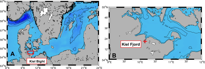
Plankton sampling was performed at the GEOMAR deck (54° 19´48´´N, 10°9´1´´E, see map in Fig. 1) between 10.00 and 11.00 h from Mondays to Saturdays in the period of August 12 to October 21, 2008. Samples of M. leidyi were taken with a WP2 net (0.8 m net opening, 500 µm mesh size), with three vertical hauls being made at each sampling occasion from the bottom (6 m) to the surface. Individuals were counted and measured alive immediately after sampling since M. leidyi disintegrate in standard fixation solutions. Total length was measured to the nearest 0.1 mm for individuals with closed lobes. Mesozooplankton were sampled at the same station at weekly intervals by using a plankton net (0.6 m diameter opening, 200 µm mesh size) from integrated vertical tows of 6 m depth to the surface. Samples were preserved in 5% buffered formaldehyde-seawater mixture for later quantification. Mesozooplankton samples were divided using a plankton splitter³⁹ until at least 100 individuals (including copepodites and adults, excluding nauplii) of the numerically dominant copepod species were found in a single subsample. All mesozooplankton specimens in the samples were identified at least to genus level under a dissecting microscope by Paulsen, Hammer, Malzahn, Polte, von Dorrien and Clemmesen⁴⁰ using the taxonomic guide by Sars⁴¹. See assemblages of mesozooplankton in Supplementary Fig. 2A and copepods in Supplementary Fig. 2B. For later counts of microzooplankton, water samples (250 ml) were taken from mid-depth on a weekly basis and were preserved using Acid-Lugol. Microzooplankton species composition was determined at least to the genus level using a convert microscope. Temperature and salinity were measured at a one-meter interval along the whole water column on each sampling day. Other environmental factors like wind direction, wind speed, and water level were obtained from a meteorological station at the roof of GEOMAR.

M. leidyi specimens were divided into two size categories, larvae and adults, according to their morphological features⁴². Small tentaculated cydippid larvae that had no sign of developed oral lobes and auricles and transition-stage larvae with tentacles and small oral lobes were ranked as larvae (1–9 mm). Specimens at the lobate stage and with developed auricles were counted as adults.

Laboratory culture experiment

To obtain direct evidence of whether adult M. leidyi consume their larvae, we performed a feeding experiment with and without ¹⁵N labeled food. Our experiment involved three trophic levels. As food for the copepod Acartia tonsa, we first cultured the cryptophyte alga Rhodomonas sp in two different treatment levels (a) labeled cultures with F/2 medium containing labeled ¹⁵N NH₄NO₃ and (b) non labeled F/2 medium. Freshly hatched nauplius of A. tonsa from GEOMAR permanent cultures were transferred to two new containers and were fed permanently with two types of Rhodomonas sp. After a month, by which time they had reached the copepodite stage of C3-4, M. leidyi larvae (size 4.6 ± 0.4 mm) were taken from the permanent cultures, kept in 20 liter buckets, and fed with two types of copepods at surplus level. Water was exchanged once a day.

All experimental organisms were kept at 15 °C, the light intensity was 100 µmol photons m⁻² s⁻¹ at a light:dark cycle of 16:8 h, and the salinity was 16. These conditions are typical for late summer conditions in the Kiel Fjord. For culturing Rhodomonas sp.⁴³, we used Provasoli’s enriched seawater medium according to Thomsen and Melzner⁴⁴. The algae were ¹⁵N-labeled by adding 0.807 g 99 atom% ¹⁵N-(NH₄)₂SO₄ (Cambridge Isotope Laboratories) and 22.011 g natural abundance NH₄NO₃ to 1000 ml of stem solution. 2 ml of stem solution were added to each litre of culture medium.

To be sure that the larvae accumulated a measurable amount of excess ¹⁵N, we fed them copepods for one week. A triplicate feeding experiment was designed in two feeding levels a) M. leidyi adults were fed with labeled M. leidyi larvae and M. leidyi adults were fed with non-labeled copepods. A total of ten larvae were transferred to a 2-liter jar with one adult M. leidyi from GEOMAR continuous culture. The adults were starved for a period of 24 h prior the experiment. The feeding experiment was terminated after 36 h. To track mortality of both M. leidyi larvae and copepods without predators, two extra units were added to the original design without predators. Adults and remaining larvae that were not used as feed were freeze-dried individually. All treatments were performed in triplicate.

Isotope analyses and biomass

For determining C and N contents, and ¹⁵N/¹⁴N ratios of the experimental M. leidyi, we transferred around 5 mg of M. leidyi dry mass into tin capsules. The samples were analyzed at Centre for Stable Isotope Research and Analysis at University of Göttingen with a Euro EA 3000 interfaced to a Delta V Plus via a Conflo IV interface. The ¹⁵N/¹⁴N ratio of atmospheric N was used as primary reference and acetanilide (C₈H₉NO, Merck, Darmstadt) was used for internal calibration.

To calculate the biomass of larvae assimilated by adults, we first calculated the mass of excess ¹⁵N in adults incubated with ¹⁵N labeled larvae:

where [N] signifies the mass of nitrogen for a given isotope, subscript e ¹⁵N-labeled adults, and subscript c ¹⁵N-unlabeled adults (the control).

Next, we estimated the biomass of larvae assimilated by adults (j) by rearranging Eq. 6 and substituting e with j:

Structural equation modeling

SEM was used to numerically assess the complex interactions between biotic and abiotic drivers of M. leidyi abundance and partition the direct and indirect effects of environmental drivers on M. leidyi seasonal growth. To partition the net effects of environmental variables on population growth and decline and their relative importance, data were separated into two groups, see Fig. 3, and analyzed in a framework of multigroup SEM. The first model assessed population growth and included abiotic (temperature and salinity) and biotic factors (micro and mesozooplankton). The second model assessed drivers of population collapse that besides the above abiotic and biotic factors included a density-dependent factor (adult abundance) with and without cannibalism. Based on previous observations¹⁷, we hypothesized that (i) M. leidyi population growth is driven by food availability, and the match with warming condition, (ii) while the population collapse may response to food depletion, temperature decline and cannibalism.

Daily ration assessment

To estimate the mean community carbon content per individual copepod, copepod abundances were transformed to micrograms of carbon using carbon contents from Supplementary Table 1. Clearance rates for adults (Cl_ad) were obtained from Granhag, Møller and Hansson⁴⁵ including a temperature regulation via Q₁₀. For copepod predation (copepod Oithona sp., size ca. 0.45 mm), this rate was used:

In the case of larvae predation, after copepod depletion (day 237), this equation was applied (gelatinous zooplankton Oikopleura dioica, 1.5 mm):

with l (mm) oral-aboral length of adults and Q₁₀ = 2.7⁴⁶.

The daily ration of adults was defined as the ingestion rate per capita (DR, % body C d⁻¹), feeding on larvae (DR_larv) or copepods (DR_cop) (Eqs. 4 and 5). The carbon content per adult (CC_ad) was defined as a function of l according to Sullivan and Gifford⁴². Larvae carbon content (CC_larv) is defined in Table 1 (0.037 mg C):

and then, ingestion (I) by adults (CC_ad) of copepods (CC_cop) or larvae (CC_larv) predation was defined as:

where A_larv and A_cop are the larvae and copepod abundances (individuals m⁻³) and an assimilation efficiency (alpha _l = 0.8) and (alpha _c = 0.4)⁴⁷. The carbon content of copepods was set to 0.9 µg C ind⁻¹, following in situ copepod assemblages (Supplementary Fig. 3).

Statistics and reproducibility

The Baltic Sea map (Fig. 1) was created with the m_map package for Matlab R2018⁴⁸. The Independent Samples T-Test for testing isotopic differences between the two treatments (n = 3) was performed in R version 3.6.1. The SEMs were run in AMOS (version 21). All SEM data were equally weighted and standardized to zero mean and unit variance. SEM was applied on a matrix of abiotic (temperature, salinity) and biotic (microzooplankton, mesozooplankton and cannibalism) factors. The strength and sign of the links and quantification of the SEM were determined by simple and partial multivariate regression and Monte Carlo permutation tests (n = 1000), whereas chi-square values were used to assess the fit of the overall path model. The individual path coefficients, i.e., the partial regression coefficients, indicate the relationship between the causal and response variables. Significance levels for individual paths between variables were set at p = 0.05. To analyze the data used for SE Ms, we compared models with the observed covariance matrix, using maximum likelihood and χ² as goodness-of-fit measures. When P < 0.05 data were considered significantly different from the model. As data from the individual groups fit the model (P > 0.05), we considered legitimate to perform a multigroup SEM analysis. Significance levels for individual paths between variables were set at α = 0.05. The daily ration assessments were generated in Matlab R2018, and the results were plotted with Sigmaplot v.14. No specific code was developed for Fig. 4.

Reporting summary

Further information on research design is available in the Nature Research Reporting Summary linked to this article.

Source: Ecology - nature.com