A system wide approach to managing zoo collections for visitor attendance and in situ conservation

A priori meta-model

SEM integrates multivariate relationships, testing both direct and indirect effects within a system²³. SEM requires a strong theoretical and empirical knowledge of the study system to guide model specification and modification²³. We conducted a literature review of the relationships between institutional attendance, zoo species composition and in situ contributions. Based on this prior theoretical knowledge and proposed causal relationships, we developed a hypothetical a priori meta-model^24,25 (Supplementary Fig. 1). This meta-model represents general relationships between multiple variables, while omitting statistical details²⁴. A thorough description of both the prior theoretical knowledge and proposed causal relationships used to generate the a priori meta-model depicted in Supplementary Fig. 1 are explained in Supplementary Note. 1. This hypothesised causal diagram was combined with available data to test the effects of species body mass on institutional attendance in the context of institutional compositional characteristics and socio-economic variables.

Data

All data generated or analysed during this study are included in Supplementary Data 1–3. Annual attendance figures and institutional area were obtained from the IZY²⁶. In the absence of available revenue data, we use visitor attendance as a proxy of income to potentially fund in situ activities. Institutional vertebrate species holdings (mammalian, avian, reptilian and amphibian) were obtained from Species360²⁷. Species360 is an international non-profit organisation that hosts and develops the Zoological Information Management System (ZIMS), the largest database of comprehensive and standardised information on >1100 zoo and aquarium collections globally. IZY and Species360 member institutions were cross-referenced and theme parks, aquariums and conservation/science centers removed to prevent potential biases, resulting in a sample size of 458 institutions in 58 countries (Supplementary Fig. 2). Safari parks and similar drive-through animal parks were treated the same as other institutions.

Both the IZY and ZIMS databases are based on submitted records from individual institutions. While these databases have not been subjected to editorial verification, potentially permitting differences in attendance calculations (e.g., exclusion of annual pass holders) or failure to update species holdings, they represent the only global databases of zoo attendance figures²⁶ and collection composition records (ZIMS). As a result, ZIMS is used by the IUCN, Convention on International Trade in Endangered Species (CITES), the Wildlife Trade Monitoring Network (TRAFFIC), United States Fish and Wildlife Service (USFWS) and Department for Environment, Food and Rural Affairs (DEFRA)²⁸.

Taxonomy and the status on the IUCN Red List of Threatened Species^TM were standardised for the 4822 vertebrate species present using the ‘taxize’ package in the statistical program R^29,30. Species richness, number of animals, taxonomic and IUCN Red List status representation, and both alpha and beta diversity indices were calculated using data from ZIMS species holdings (see Table 1 for variables list).

Species body mass was obtained from the Species Knowledge Index³¹, which standardises data across 22 different global demographic databases. Species-level body mass information was available for 4214 species. Body mass for the remaining 608 species was inferred at the genus, family or order level using the same datasets. This allowed the mean species body mass of each institution to be calculated as shown in Eq. (1).

Where (bar M) is the mean abundance weighted species body mass per institution, x_i is the number of individuals of species i, m_i is the body mass of species i, where i goes from 1 to n species per institution.

To assess socio-economic factors, we used GDP and national population size for each country³². Institutional GPS co-ordinates were used to calculate total population sizes within 10 km radii in ArcGIS using estimated global population counts³³.

In order to assess the in situ contributions of individual institutions the AZA Annual Report on Conservation and Science was consulted³⁴. This provided the number of field conservation programmes, in which AZA member institutions were involved in 2015. When cross-referenced with IZY and Species360 members, this provided a sample size of 119 institutions across four countries for which we could analyse in situ contributions. The number of projects, as a measure of in situ conservation contributions, does not provide further resolution on the form the contribution takes (e.g., financial, expertise, resources, animals, training, etc.). However, a separate analysis of the relationship between the number of in situ projects supported and the total in situ financial investment per institution was conducted on anonymised data from 83 individual British and Irish Association of Zoos and Aquariums (BIAZA) institutions. These data show a clear positive relationship between the number of in situ projects supported and total in situ financial expenditure. As this data set was anonymised, we were unable to include it in our integrated model; however, these data are shown in Supplementary Fig. 5 and support our assumption that the number of in situ projects is a meaningful proxy for the total in situ financial investment per institution.

Analyses

Two distinct SEM frameworks were tested, the attendance model and the in situ model. The attendance model tested the relationship between visitor attendance and all the various specified variables for 458 institutions globally. This model did not include any in situ contribution data. The in situ model tested the relationship between visitor attendance, in situ contributions and all the various specified variables for a subset of 119 institutions in North America for which in situ contribution data were available. The results of the attendance model were used to guide the development of the attendance linked pathways in the in situ model as the larger sample size of the attendance model had higher power. The results of the attendance model are combined with the results of the in situ model in Fig. 2, with a yellow box delineating the boundary of the two models. Only the additional in situ pathways of the in situ model are reported, as all other relationships were derived from the attendance model due to its higher statistical power.

All analyses were carried out using the R program (version 3.4.3) and the packages ‘lavaan’³⁵ and ‘lavaan.survey’³⁶ for SEM. All variables were both mean centered and expressed in units of standard deviation to allow direct comparisons of effect sizes between variables.

Attendance model

We combined prior theoretical knowledge and proposed causal relationships to create the a priori SEM meta-model (Supplementary Fig. 1 and Supplementary Note. 1). The meta-model captured all evidence-based relationships that we found in our literature review and all plausible and suspected predictors of attendance that we hypothesised. This model was then refined to create the final model depicted in Fig. 2 using the approach described in Grace et al.³⁷and similar to that implemented in Grace et al.²⁵. In summary, the a priori meta-model was modified through addition and deletion of pathways using model-data fit procedures to produce a range of plausible alternative models which were compared using corrected Akaike’s Information Criterion (AICc) values. All modifications to the model, with pathways removed or inserted, were based on quantitative recommendations, theoretical intuition and model-data fit. Model-data fit was assessed using a combination of absolute fit indices (e.g., Standardised Root Mean Square Residual) and incremental fit indices (e.g., Comparative Fit Index), to account for the differential sensitivity of fit indices to data distribution, model size and sample size³⁸. Modification indices were used to guide the addition of suspected pathways, with a standard cut-off level for the chi-square test criterion of 3.84³⁹. Highest value modification indices were considered first, however, as modification indices do not take into account whether or not relationships make theoretical sense, intuitive theoretical relationships were also considered, as outlined in the Supplementary Code provided. Following the addition of these pathways, p values were then used to identify potentially unsupported pathways, with a threshold of 0.05. Highest p values were considered first for removal. Overall model selection from the pool of competing models was achieved using AICc values⁴⁰, with a threshold of more than two AICc units lower than the nearest competing model being considered sufficient for model selection. The AICc values of competing models are shown in Supplementary Table. 1. The final selected attendance model was validated, using four random subsets of the existing data (n = 200 each time), to ensure parameter estimates were similar when using different datasets from the same sample²³. Institutions were included within countries in the model.

In situ model

Due to the lower sample size in the in situ model, which only covered four countries, we did not include GDP and country as variables. We started with the most complete model to predict both in situ contributions and attendance. Initial attendance links were based on the results of the best attendance model. Model-data fit and model selection were assessed in the same manner as for the attendance model.

Tests of mediation were performed on mediated pathways to ensure both direct and indirect effects of variables were justified in both models. Values for both Absolute Fit Indices and Incremental Fit indices were supportive of good model fit (Supplementary Table. 2). All standardised path coefficients, total effect sizes, significance values and proposed interpretations of causal pathways for both models are shown in Table 2. See Fig. 3 for bivariate relationships between attendance, in situ contributions and their strongest predictors. These models incorporate species abundance per institution, however, models using species presence–absence only were also assessed and provided overall similar results and conclusions, with qualitative differences found in only four links per model (see below). An updated meta-model reinforces many previously supported relationships, such as those between species body mass, species richness and the number of animals present (Supplementary Fig. 3).

Fig. 3: Bivariate relationships between institutional attendance, in situ contributions and their strongest predictors.

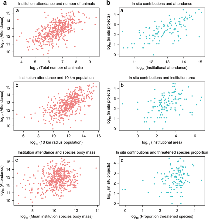
a (left panel, n = 458), log₁₀ transformed bivariate plots of institutional attendance and total number of animals, 10 km radius population and mean species body mass a–c. b (right panel, n = 119), log₁₀ transformed bivariate plots of institutional in situ contributions and attendance, institutional area and the proportion of threatened species present per institution a–c. All variables are adjusted for species abundance per institution. Source Data: Supplementary Data 1 and 2 provided.

Full size image

Species presence–absence SEM frameworks

The attendance and in situ model results reflecting species presence–absence only are shown in Supplementary Fig. 4. Chi-squared statistics, fit indices, standardised path coefficients and proposed interpretations for both the attendance and in situ models reflecting species presence–absence are also presented (Supplementary Tables 3 and 4). Residual covariances for both the attendance and in situ models are shown in Supplementary Table. 5 (species abundance models) and Supplementary Table. 6 (species presence–absence models).

Reporting summary

Further information on research design is available in the Nature Research Reporting Summary linked to this article.

Source: Ecology - nature.com