Ethical Statement
Schilbe intermedius is not protected under any legislation and not considered threatened or endangered. Samples from Nigeria were collected from non-protected areas for which permissions were not required as the sampling locations do not fall under the Nigerian Wildlife Protection Act.
Sample collection
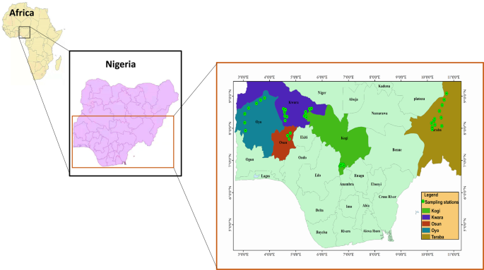
With the help of local fishermen and field assistants, 118 individuals of S. intermedius were collected from different freshwater bodies in Nigeria (Table S1) between July to December 2018. Individuals were collected using gill nets, hook and line, and/or cast net, and transported on ice to the Zoology Laboratory of the Department of Bioscience and Biotechnology, Kwara State University (KWASU), Malete, Nigeria. The preliminary species identification was in accordance with the taxonomic guidelines2,31,32. Additional species identification and verification were carried out by two trained taxonomists at the Department of Zoology, University of Ilorin, Nigeria. Tissue (tail fin) samples were collected and preserved in 95% ethanol and subsequently stored under −80 °C at the State Key Laboratory of Genetic Resources and Evolution, Kunming Institute of Zoology, Chinese Academy of Sciences, China. Vouchers were fixed with 4% formalin and kept in 70% ethanol for long-term storage at the Zoology Laboratory of the Department of Bioscience and Biotechnology, KWASU, Nigeria.
DNA extraction, PCR amplification, and sequencing
Total genomic DNA was extracted from the ethanol-preserved tissues following the standard phenol-chloroform extraction procedure after digestion with proteinase K33. The COI gene fragment of the newly acquired specimens was amplified with primers7 in a volume reaction of 25 µl: 1.5 µl of genomic working DNA, 18.5 µl of PCR water, 2.5 µl of PCR buffer, 2 µl of dNTP, 1 µl of each of the forward and reverse primers (10 pm/µl) and 0.30 µl of rTaq polymerase. The PCR cycle profiles were as follow: 5 minutes initial denaturation at 94 °C, followed by 35 cycles of 1 minute at 94 °C, annealing for 45 seconds at 55 °C, an extension for 1 minute at 72 °C; final extension for 10 minutes at 72 °C. Purified PCR products were directly sequenced in both forward and reverse directions with an automated DNA sequencer (ABI 3730).
DNA sequence alignment and dataset assembly
To confirm the identity of the amplified sequences, sequences were submitted to BLAST searches in National Center for Biotechnology Information- NCBI (https://blast.ncbi.nlm.nih.gov/Blast.cgi). Thereafter, 101 COI sequences of S. intermedius from West, South, East and Central Africa were downloaded from the NCBI (http://www.ncbi.nlm.nih.gov) and Barcode of Life Database (http://www.boldsystems.org/index.php/TaxBrowser_Home) (Table S1). Further, COI sequences of five closely related species (Schilbe mystus, Schilbe multitaeniatus, Schilbe grenfelli, Schilbe marmoratus, and Schilbe zairensis) were downloaded as outgroup taxa (Appendix 1). A total of 219 COI nucleotide sequences of S. intermedius and five outgroup taxa were aligned in MEGA 7.034 using ClustalW35 with default parameters. The aligned sequences were translated into amino acids using the vertebrate mitochondrial code and no premature stop codons were observed, suggesting that the open reading frame was maintained in the protein-coding loci.
Phylogenetic reconstruction and species delimitation tests
For the phylogenetic reconstruction, the sequence dataset was collapsed into 31 unique COI haplotypes of S. intermedius using DnaSP 5.1036. MtDNA phylogeny was reconstructed using Bayesian Inference (BI) and Maximum Likelihood (ML) approaches. The best partition strategy and nucleotide substitution model for the BI were selected using the Akaike information criterion (AIC) as implemented in PartitionFinder 1.0.137. Following analysis using Partition Finder, the mtDNA COI sequence dataset was partitioned into codon 1, 2 and 3, and the best-fitting models were selected for each of the partitioned data. For BI analysis, four independent Markov chain Monte Carlo Chains (MCMC) were run simultaneously for 10 ×106 generations with sampling every 1000th generation) as implemented with MrBayes 3.1.238. Two runs were conducted independently, and the first 25% of the tree discarded as burn-in. The ML was performed, under model GTR + G as evaluated in PartitionFinder37, with 100 random addition replicates and per partition branch lengths39 as implemented in RAXML v. 7.0.340. The reliability of the ML tree was assessed by bootstrap analysis41 including 1000 replications. The resulting BI and ML trees were visualized using FigTree v1.4.242. Bayesian Posterior Probabilities ≥ 0.95 for BI and bootstrap proportions ≥ 70% for ML were considered strongly supported. To visualize the relationships between haplotypes, a haplotype network was constructed using the median-joining algorithm43 implemented in Network 5.0.1.1 (www.fluxus-engineering.com).
To estimate the likely number of species units within S. intermedius, three different species delimitation approaches were employed:
In approach 1, species unit was assessed with TaxonDNA 1.8 with the ‘Cluster’ algorithm implemented in SpeciesIdentifier44. This method considers overlaps between the intra and interspecific variation, and the maximum pairwise distance within recognized putative species-level criterion should not exceed a given threshold. Species unit, herein termed clusters, are identified according to pairwise (uncorrected) distances for sequences within each cluster. We reduced the dataset to include the 31 unique haplotypes of S. intermedius previously identified. Incremental values ranged from 1.0% with an increase of 0.5% in each step to a maximum of 3.0%.
In approach 2, the automatic barcode gap discovery (ABGD)45 was performed on the online server (http://wwwabi.snv.jussieu.fr/public/abgd/) using all 220 sequences of S. intermedius. ABGD sorts the terminals into hypothetical species with calculated p-values based on the barcode gap. ABGD analyses used Kimura 2-parameter (K2P) and Jukes-Cantor (JC69) distances with setting parameters: Pmin = 0.001, Pmax = 0.2, relative gap width = 1.5 and Nb bins (for distance distribution) = 20, with the other parameters at default values.
In approach 3, PTP analyses were conducted on the bPTP web server (http://species.h-its.org/ptp/) using the RAxML tree of the unique haplotypes as input data (out-groups removed before analysis) with 100,000 MCMC generations, thinning set to 100, burn-in at 25% and performing a Bayesian search. The probability of each node to represent a species node was calculated using the maximum likelihood solution.
Population genetic analyses and historical demography
Since genetic diversity is reflected by the measurement of nucleotide diversity (π) and haplotype diversity (h), we computed the number of haplotypes (H), haplotype diversity (h), nucleotide diversity (π) and mean number of pairwise differences (k) for each matriline using DnaSP. The historical demographics of the matrilines of S. intermedius were evaluated using arrays of statistics: First, mismatch distributions46 were calculated with Arlequin 3.547 and used to examine signals of population expansion or stability over time. We assumed population stability would generate multimodal distribution, while expansion would imply unimodal pattern48. We compared observed distributions of nucleotide differences between pairs of haplotypes with those expected under spatial49 and demographic47 expansion models by using the generalized least square approach. In addition, we used the sum of squared deviations (SSD) as goodness-of-fit statistics for the observed and expected mismatch distributions, and the significance of fit for expansion model was tested, while the confidence intervals for the associated parameters estimates using 1000 bootstrap replicates were examined. Secondly, for the neutrality test, Tajima’s D50, Fu and Li’s D, and F51 tests were conducted for each matriline using Arlequin. Our assumption is that, if population sizes had been stable across time, Tajima’s D and Fu and Li’s D would be near zero. However, we assumed that significantly positive values would be expected in populations that experienced recent bottlenecks, and significantly negative values imply the recent population expansions50,51. We also computed Fs52 since causation is difficult to ascertain when Tajima’s D deviates significantly from zero. This statistic is particularly useful for detecting population expansions. We also assumed that a negative value of Fs implies recent population expansion or genetic hitchhiking, while a positive value results from a recent population bottleneck.
Source: Ecology - nature.com
