Study location and field methods
We attached either light-level geolocator or Global Positioning System (GPS) tags to adult Swainson’s Thrushes in breeding condition in coastal California, and in the Tahoe and Lassen regions within California’s northern Sierra Nevada and southern Cascade Mountains (hereafter the Cascade-Sierra), in the summers of 2014–2015 (Fig. 1; Supplementary Table S1). Light-level tags collected light-intensity data from which latitude and longitude were coarsely estimated, and GPS tags were programmed to collect 8 positions from satellites, spanning the winter period. In the coastal region, we deployed tags in the San Francisco Bay area: 10 light-level tags south of San Francisco Bay in coastal San Mateo County in 2014, and 30 GPS tags north of the bay in the Point Reyes area of Marin County in 2015. This was the second phase in this effort in the Point Reyes area: light-level tags were previously deployed in 201022, and those data are included in the results presented here. In the Cascade-Sierra, a mix of light-level and GPS tags were deployed in each of two regions: 11 light-level and 10 GPS tags in the Lassen region in the northern Sierra Nevada/southern Cascade Mountains, Plumas County, in 2015; and 24 light-level and 5 GPS tags farther south in the Tahoe region of the northern Sierra Nevada, Placer and El Dorado counties, in 2014 and 2015. On the coast, tag deployment and recovery was primarily done during normal operations at constant-effort mist-netting stations; and in the Cascade-Sierra, tag deployment and recovery was done via target netting, using song playback and decoys. Due to the differences in capture methods among the regions, sex ratios on the coast were fairly equal, whereas they were strongly male-biased in the Cascade-Sierra. See Supplementary Table S1 for more tagging details by location. The habitat at capture sites on the coast included riparian forest and Douglas-fir (Pseudotsuga menziesii) forest mixed with coastal scrub23,24, and in the Cascade-Sierra was dominated by dense riparian vegetation and wet riparian mountain meadows.
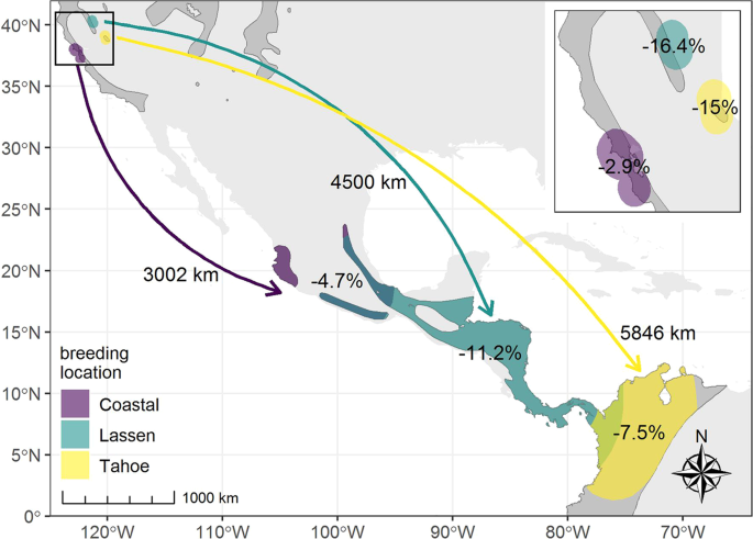
Estimated wintering destinations, relative forest loss (from 2000–2017)32, and migration distances for three breeding populations of Swainson’s Thrush in California. Dark gray polygon (often not visible beneath colored areas) indicates estimated breeding and winter ranges31; note, the authors know of additional breeding sites slightly beyond these boundaries, including where Lassen birds were tagged (see Supplementary Fig. S1); and the open polygon in middle of the Lassen wintering range is considered outside the known wintering range of the species. Dark teal reflects the area of potential overlap in wintering ranges of coastal and Lassen birds, and yellowish-green the area of potential overlap between Lassen and Tahoe birds. Exact breeding tag-deployment locations are buffered to quantify regional forest loss at a more appropriate scale, and wintering destinations reflect 95% kernel densities to account for estimations involved in light-level technology. Arrows connect corresponding breeding and wintering areas, and distances shown between breeding and wintering areas, represent great-circle distances between the centroids of each polygon; neither are intended to imply migratory routes.
Light-level tags (developed by British Antarctic Survey or Migrate Technology Ltd) and PinPoint8 GPS tags (developed by Lotek Wireless) were attached with a leg-loop harness25 of StretchMagic jewelry cord of 1.0 mm gauge (light-level tags) or 0.7 mm gauge (GPS tags), and each harness sealed with a small crimped jewelry bead and super glue. The average weight of the harness and GPS tag together was 1.0 g, averaging 3.4% of the bird’s weight (n = 37); the average weight of the harness and light-level tag together was 0.8 g, averaging 2.8% of the bird’s weight (n = 18). Each bird was banded with a federal U.S. Geological Survey aluminum band; additionally, those in the coast and Lassen regions were also given either a unique or cohort color band, and those in the Tahoe region a unique combination of three color bands and one federal band. We determined age of each bird (only adults were tagged), determined sex using the presence of a brood patch (female) or cloacal protuberance (male), and weighed each bird to the nearest 0.1 g before and after the geolocator tag was attached. The technology requires recapturing birds following a full migration cycle, upon which we removed the tags, extracted the data, and collected the same information (age, sex, weight) as during the initial capture. Recovery occurred the following two spring/summer seasons after deployment. Capture and handling followed strict bird safety protocols in accordance with the North American Banding Council26. All banding and tagging was approved by the United States Geological Survey’s Bird Banding Laboratory (USGS BBL Permit Numbers: 09316 and 23272).
Analysis
Daily location estimates (GPS tags)
We programmed the GPS tags to attempt to collect 8 GPS coordinates during the wintering period between 25 October and 25 March (date range based on previously-determined wintering arrival and departure dates22), to attempt to determine their wintering locations and potential within-winter movements22,27. We downloaded location estimates from recovered GPS tags using Lotek Wireless PinPoint Host software, revision 3 (2014). For tags with multiple (2–6) points, we used the mean latitude and longitude estimates; the maximum distance between points for a given individual was 2.8 km.
Daily location estimates (Light-level tags)
We used IntigeoIF software version 1.5.2 (Migrate Technology) to download the light intensity data. To analyze the data, we log-transformed the light values, and used the TwGeos package28,29 to identify twilight events. We then analyzed the light-level data with a Bayesian framework using the Solar/Satellite Geolocation for Animal Tracking (SGAT) package30; SGAT uses the twilight times calculated using the threshold method, the observed difference between the known twilight times and those calculated, and a movement model.
To identify twilight periods, we used a threshold value of 0.65 for all individuals; we selected a threshold as low as possible, but above most of the noise in the nighttime light levels. We used the twilightEdit function to delete twilights (sunrise/sunset events) if they occurred 15 min before or after the previous or next day’s twilight value; we used a 4-day window (2 days before and after), and set stationary site variation to 20 minutes28.
We used two on-bird calibration periods for each tag: the first calibration period was from the day after tag attachment to 31 August of the tagging year, before the bird departed for fall migration. The second calibration period began the year after deployment on 5 June, after which all birds appeared to be back on the breeding grounds, and ended the day before the bird was recaptured. For two birds, the tag failed before spring migration, so only the first calibration period was used. We estimated the zenith angle for each tag; the zenith angle is defined as the angle of the sun relative to the earth’s 90° vertical axis, when the light intensity data from the geolocator crosses a specific threshold (e.g., set at 0.65 for our tags). Using the defined calibration periods above, we estimated median zenith angles for each tag (range 94.8° to 96.5°), and used each tag’s estimated zenith angle to plot estimated positions for the entire tag deployment period.
For the SGAT analysis we used a movement model with probable flight speeds defined by a gamma distribution (mean of 2.2 and a SD of 0.25). We also used a land mask which limited the bird’s location to land during stationary periods. To generate the posterior distribution, we used 3 independent chains, 6000 samples for burn-in and tuning, and then based our analyses on a final run of 1000 samples.
For each individual, we checked that location results were relatively consistent between the simple threshold location estimates and the subsequent modeled estimates. We also checked that location estimates were not sensitive to small changes in model assumptions. Through this process, we excluded one tag for which wintering areas varied from as far north as Cuba to as far south as Peru depending on minor variations in the analysis method.
Mapping breeding and wintering regions
We estimated the wintering regions for each breeding population (coastal, Lassen, and Tahoe) by creating a 95% kernel density estimate around all known (GPS) and estimated (light-level geolocator) wintering locations for both tag types. Similarly, we created a 95% kernel density estimate around all the known breeding tag deployment locations and further buffered these small areas by 20 km, to better capture the surrounding landscape and quantify regional forest loss at a more appropriate scale.
Estimating forest loss
We clipped all breeding and wintering polygons to the published species range31 to allow us to focus our consideration of habitat change to the area within the species range. We then estimated relative landscape-level forest loss in each of these polygons separately using 2000–2017 data available from Global Forest Change32. The data are divided into 10×10 degree tiles with a spatial resolution of 1 arc-second per pixel (equivalent to approximately 30 m at the equator). Separate tiles contain information about the baseline canopy cover in the year 2000 (“baseline”) and the year in which any forested pixel became unforested (“lossyear”). We converted baseline cover from the year 2000 into a binary (0 or 1) reflecting whether or not each pixel was forested, using a minimum threshold of 50% forest cover. For each pixel forested in 2000, we also converted “lossyear” data into a binary (0 or 1) reflecting whether or not each pixel became unforested by 2017. For all pixels within each Swainson’s Thrush wintering area polygon, we summarized the number of pixels where forest was originally present in 2000, and the proportion of those pixels where forest was lost by 2017. Forest growth data were also available, but only through 2012; we assumed that 12 years was a relatively short time frame within which an unforested pixel could become forested, and therefore we ignored forest gains in this analysis.
Measuring migration distance
As a conservative index of migration distance, we measured great-circle distances between the centroids of each breeding area polygon and its corresponding wintering area polygon. We do not know the actual route taken nor exact distances flown by each individual bird.
Source: Ecology - nature.com
