Regulatory relationship between quality variation and environment of Cistanche deserticola in three ecotypes based on soil microbiome analysis

Study site description and sampling

According to field investigations, C. deserticola has three main ecotypes, including saline-alkali land, grassland and sandy land. In April, 2017, we collected soil samples representing the major ecotypes of C. deserticola in China. Soil samples of saline-alkali land were collected from Ebinur Lake (AB1, AB2, AB3) andBaicheng Beach (BJ1, BJ2, BJ3, BJ4, BJ5) in Xinjiang province. Grassland soil samples were taken fromTula Village (TL1, TL2, TL3, TL4, TL5) in Xinjiang province. Soil samples of Sandy land were collected from Alxa (AL1, AL2, AL3, AL4, AL5, AL6) in Inner Mongolia province and Minqin county (GS1, GS2), Changcheng county (GS3, GS4) in Gansu province. The longitude, latitude and altitude information of all sampling points are shown in Table 1 and Fig. 1. At the field site, we used a stainless steel cylindrical drill with a diameter of 5 cm to collect the soil adjacent to the succulent stem of C. desertica and its host, and immediately stored it in a portable refrigerator at –20 °C. After transport to the laboratory, the soil samples were passed through a 2-mm sieve to remove plant tissues, roots, rocks, etc. and stored at –20 °C in a refrigerator before further experiments.

Figure 1

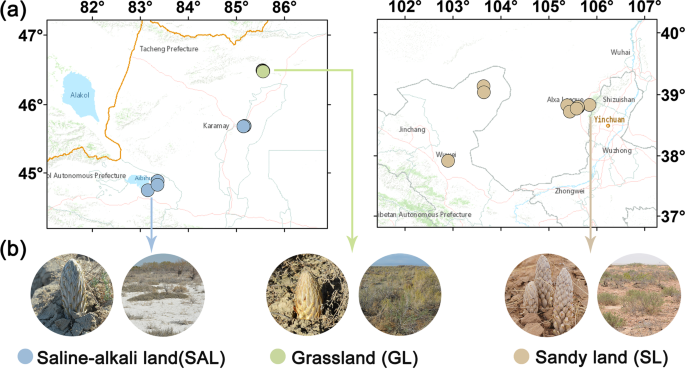
Soil sampling points map and close-up photos of plants C. deserticola in saline-alkali land (SAL), grassland (GL) and sandy land (SL).

Full size image

DNA Extraction and 16S rRNA Sequencing

Soil DNA was extracted using the PowerSoil DNA Isolation Kit (MoBio Laboratories, Carlsbad, CA) following the manual¹². The purity and quality of the genomic DNA were checked by 0.8% agarose gels electrophoresis and nanodrop.

The V3-V4 hypervariable region of bacterial 16S rRNA gene was amplified with the primers 338F (ACTCCTACGGGAGGCAGCAG) and 806R (GGACTACHVGGGTWTCTAAT)¹³. For each soil sample, a 10-digit barcode sequence was added to the 5′ end of the forward and reverse primers (Allwegene Company, Beijing)¹². The PCR was performed on a Mastercycler Gradient (Eppendorf, Germany) using 25 μl reaction volumes containing 12.5 μl KAPA 2G Robust Hot Start Ready Mix, 1 µl forward primer (5 µM), 1 µl reverse primer (5 µM), 5 µl DNA (total template quantity is 30 ng) and 5.5 µl H₂O. The cycling parameters are as follows: 95 °C for 5 min, followed by 28 cycles of 95 °C for 45 s, 55 °C for 50 s and 72 °C for 45 s, with a final extension at 72 °C for 10 min. Three PCR products per sample were pooled to mitigate reaction-level PCR biases. The PCR products were purified using a QIAquick Gel Extraction Kit (QIAGEN, Germany) and then quantified using real-time PCR¹⁴.

Deep sequencing was performed on a MISeq platform at the Allwegene Company (Beijing). After the run, image analysis, base calling and error estimation were performed using Illumina Analysis Pipeline Version 2.6¹⁴.

Data analysis

The raw data were firstly screened, and sequences were removed based on the following considerations: sequences shorter than 200 bp with low quality score (≤20) and contained ambiguous bases or did not match the primer sequences and barcode tags¹⁵. Qualified reads were separated using the sample-specific barcode sequences and trimmed with Illumina Analysis Pipeline Version 2.6. Then, the datasets were analysed using QIIME. The sequences were clustered into operational taxonomic units (OTUs) at a similarity level of 97%¹⁶ to generate rarefaction curves and calculate the richness and diversity indices. The Ribosomal Database Project Classifier tool was used to classify all sequences into different taxonomic groups¹⁵. Clustering analyses were performed based on the OTU information from each sample using R to examine the similarity between different samples¹⁷. The UniFracdistances matrix between microbial communities from each sample were calculated using the Tayc coefficient and represented as an unweighted pair-group method with arithmetic mean clustering tree, which describes the dissimilarity (1-similarity) amongst the multiple samples¹⁸. A Newick-formatted tree file was also generated through this analysis. Alpha diversity was applied in the analysis of the complexity of species diversity for a sample using four indices, including Chao1, observed species, phylogenetic diversity (PD) whole tree and Shannon diversity index. These indices were calculated using the QIIME software (Boulder, CO, USA) in Python (v.1.8.0) (La Jalla, CA, USA)¹⁹. Beta diversity analysis was used to evaluate differences of samples in terms of species complexity. Beta diversity was calculated using the principal coordinate analysis (PCoA) and cluster analysis in QIIME²⁰. The analysis of molecular variance (AMOVA) was performed using mothur. EdgeR was used to calculate the OTU difference between groups. Heatmap.2 was used to draw the heat map, whilst Ggplot was used to draw the Manhattan map.

Determination of biomarker and core microbiome

The linear discriminant analysis (LDA) and random forest (RF) methods in the Microbiome Analyst website²¹ was used to determine the biomarker microbiome. The website firstly performs non-parametric factorial Kruskal–Wallis sum–rank test to identify features with significant differential abundance considering the experimental factor or class of interest, followed by LDA to calculate the effect size of each differentially abundant features²¹. The features are considered significant based on their adjusted p-value. The default adj.p-value cutoff = 0.05. RF analysis is performed using the randomForest package5. RF is a supervised learning algorithm that is suitable for high-dimensional data analysis. This method utilises an ensemble of classification trees, each of which is grown via random feature selection from a bootstrap sample at each branch²². Core microbiome analysis was adopted from the core function in the R package microbiome by Microbiome Analyst (https://www.microbiomeanalyst.ca/MicrobiomeAnalyst/home.xhtml).

Correlation analysis of key microbial communities, PhGs content and ecological factors

The contents of seven phenylethanoid glycosides (PhGs) of the three ecotypes of C. deserticola, namely, echinacoside, cistanoside A, acteoside, isoacteoside, 2′-acetylacteosid, tubuloside A and cistanoside F, were determined through HPLC. The chromatographic conditions involve a Waters C18 column (150 mm × 3.9 mm, 4.6 μm), and the mobile phase comprises acetonitrile and 0.2% formic acid. The chromatographic settings were as follows: 0–10 min, 10%→15% A; 10–30 min, 15%→40% A. The flow rate was 1 mL/min. The absorption wavelength, injection volume and column temperature were 330 nm, 10 μL and 27 °C, respectively. The methodology study refers to the preliminary experimental work of the reference group¹.

This study collected 16 meteorological stations near the three ecological types of C. deserticola (http://data.cma.cn/): Xinjiang Bole 51238, Tacheng 51133, Tori 51241, Karamay 51243, Buxail 51156, Yumin 51137, Emin 51145, Gansu Minqin 52681, Yongchang 52674, Wuwei 52679, Gulang 52784, Inner Mongolia Suikou 53419, Hangjinhouqi 53420 and Wuhai 53512. Data of seven climatic factors from 1981–2010 served as the climatological factor data for subsequent correlation analysis.

Redundancy analysis of differential metabolites and bioclimatic factors was performed by using Canoco 5 software²³. Pearson correlation coefficient was calculated for biomarker microbiome abundance, compound content and ecological factor data integration. In this study, the log₂ data conversion was uniformly performed before the analysis. SPSS was used to calculate the Pearson correlation coefficient of the six biomarkers, six core microbiomes, seven main active components of C. deserticola and the ecological factors in the three habitats, and the screening standard was as follows: pearson correlation coefficient (r) >0.5 and p value < 0.05. The relationships amongst the above factors were visualised using Cytoscape²⁴ (The Cytoscape Consortium, San Diego, CA, USA, version 3.7.0) and pheatmap (R package).

Prediction of the microbial functional profiles of the microbiome

Tax4Fun²⁵ (R package, http://tax4fun.gobics.de/) was used to predict the microbial functional profiles of microbiomes in the soil samples. The OTU Biom table of soil microbiome was used as an input file for the metagenome imputation of C. deserticola soil samples. Then, the predicted gene class abundances were analysed at the KEGG Orthology (KO) group level 3. The results from Tax4Fun were analysed in doBy (R package)²⁶.