Sinking flux of particulate organic matter in the oceans: Sensitivity to particle characteristics

Preliminaries: A single, sinking, remineralizing particle

We start by considering a single particle, sinking vertically through the ocean at its terminal velocity, w_sink. Several early experiments on oceanic particles attempted to characterize sinking rates¹⁴ using Stokes’ Law^15,16. While departures from Stokes’ theory result from particle shapes deviating from spherical, variations in structural from, porosity, rigidity and drag¹⁷, an assumption of Stokes’ Law is frequently applied to modern flux parameterizations^{10,18,19,20,21} and is used here with cognizance of its limitations.

For a particle of radius 1 mm, a typical sinking speed of 100 m d⁻¹, and the kinematic viscosity of water at room temperature, the particle Reynolds number is about 1. At low particle Reynolds number, and making the reasonable assumption that particle sinking is in quasi steady state, individual spherical particles have a sinking velocity w_sink, described as the balance between the downward gravitational force and the upward Stokes’ drag as

where a is the effective particle radius, μ is the dynamic viscosity of the fluid, g is the acceleration due to gravity, and ρ_p and ρ_f are the densities of the particle and surrounding fluid, respectively. The kinematic viscosity μ varies between 0.8 × 10⁻³ and 1.7 × 10⁻³ kg m⁻¹s⁻¹ derived from the range of typical temperature and salinity observed throughout the global ocean²². For this analysis we use μ = 1 × 10⁻³ kg m⁻¹s⁻¹ The characterization of particle size, sinking and remineralization in terms of an effective radius a is an assumption that permeates through the development of this model. While it is recognized that a majority of marine particles are non-spherical, such a characterization facilitates quantification and a simple analytic form. To treat a greater variety of particle shapes, we later use the fractal dimension as a way to account for complex particles.

Our model assumes that particles are colonized by bacteria upon leaving the base of the euphotic zone and are consumed steadily thereafter. At first order, the depth to which a particle will sink is therefore a balance between its sinking velocity and the rate at which it is remineralized r (per day, expressed as d⁻¹). This rate depends on several factors including, but not limited to, the particle constituents, shape, porosity and surface area available for bacterial colonization²³, the ambient temperature²⁴, microbial respiration rates²⁵, and can vary in time and space²⁶. For this study we use a range reported in Iversen et al.^27,28, with an average carbon-specific respiration rate of individual aggregates r = 0.12 ± 0.03 d⁻¹ in a 15 °C treatment, and r = 0.03 ± 0.01 d⁻¹ in a 4 °C treatment, corresponding to a life-span (r⁻¹) of approximately 8 days and 33 days, respectively.

The functional form of bacterial solubilization likely depends on the particle surface area available, the degree of colonization and hence the degree of anoxia within a sinking particle, among other ambient factors such as temperature and oxygen concentration¹³. We propose a generalized form dV∕dt ~ − raⁿ, which allows the particle volume V (and thus, mass) to diminish with time in a few ways: (a) at a constant rate (n = 0), suggesting that there is a fixed pace of remineralization irrespective of particle size, (b) proportional to the surface area (n = 2) suggesting that only the external surface of a (roundish) particle is being remineralized and that the number of bacteria (and thus the rate) decrease as the available surface area is reduced (likely appropriate for a very compact particle, or one that has an anoxic interior), or (c) proportional to the particle volume (or mass) (n = 3) suggesting that the bacteria have colonized the interior and exterior of the particle (likely appropriate for aggregates that are more like a sponge than a compact sphere). The case (c) was considered by DeVries et al.¹⁰ and Cram et al.¹³. The generalized expression for the rate of change of the particle radius is:

where C is a constant that relates to the form of remineralization. For the following derivation, we use the intermediate case n = 2.

We relate the particle density ρ_p to the fluid density at the base of the euphotic zone (ρ_T) using a dimensionless factor α as

The range of α we anticipate based on excess density observations from the literature is reported in Table 1. Assuming a linear change in density with depth β (units m⁻¹), and assuming incompressible particles (see the section Particle Compressibility), we write the fluid density ρ_f at any depth z in terms of ρ_T as

Our model parameters thus far are α, β and remineralization rate r. Substituting 4 and 3 into 1, and using the n = 2 remineralization equation, the depth- and time-dependent particle sinking velocity becomes

Integrating from the initial particle location at the base of the euphotic zone, taken to be z = 0 at time t = 0, to some depth z and time t, we arrive at the solution for the particle depth as a function of its volume (V(t)=frac{4}{3}pi {[{a}_{0}(1-rt)]}^{3}) as

The particle volume, as a function of depth, is therefore

As conceptualized, (6) predicts that the particle descends quickly at first, but slows as it is remineralized and as the relative difference between the particle and fluid density diminishes (Fig. 2a). The particle eventually disappears as V(z) approaches zero (dashed line in Fig. 2a) at depth

Figure 2

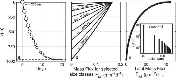
(a) A particle (a_o = 250 μm, α = 0.03) slows as it sinks into denser water (β = 5 × 10⁻⁶ m⁻¹) and is remineralized (r = 0.11 d⁻¹), until disappearing at z_dis = 980 m (Eq. 8). (b) Mass flux profiles (Eqn 9, given the initial size spectrum shown in the inset of panel c, and N_o = 10⁴ particles m⁻²d⁻¹) for particle size classes ranging from a_o = 10 to 250 μm. (c) The total mass flux (eqn 11). Note that for our model, z = 0 represents the base of the euphotic zone.

Full size image

Sinking flux for particles of single size

The total particle flux is the sum of a population of particles all undergoing a similar fate. In steady state, for particles of initial radius a_o raining down from z = 0 at a rate of N_o particles per m² per day, the depth-dependent mass flux F_M(z, a₀) is the product of N_o (which is depth independent under the assumption of steady state) and the mass (M) of an individual particle at depth z given by M(z) = ρ_pV(z). This is valid until the particle disappears, and hence

Two relevant depths can be derived from these equations: the disappearing depth (z_dis) given by eqn (8) and the suspension depth (({z}_{susp}=frac{alpha }{beta })) where a particle becomes neutrally buoyant. We find that under typical oceanic conditions and particle traits listed in Table 1, z_susp≫ z_dis, and so particles are far more likely to be remineralized before reaching a neutral density. By extension, for most z≤z_dis, the term (frac{beta }{alpha }zll 1). Hence, by Taylor expansion, the mass flux is, to good approximation, a linearly decreasing function of depth (as seen in Fig. 2b)

This solution demonstrates that a single size class of identical particles does not reproduce the canonical Martin curve flux profile (Fig. 2b). We show in the following section, that a range of particle sizes (or types) is required to generate the canonical concave downward flux profile.

A range of particle sizes and types

Among the most widely reported characteristics of oceanic particles is the vast abundance of small particles relative to larger particles^19,29. When plotted on a logarithmic scale, the particle number spectrum has a negative slope p (the ‘number spectral slope’), suggesting that particle sizes are distributed according to a power-law^{18,30,31,32,33}. This slope has been observed to vary widely, regionally, in time, and with depth, generally ranging between p = −4 and p = −2 (Table 1)¹⁹. Since the volume (and mass) of particles scales as M ~ a³ for spherical particles, a steep slope (p < −3) indicates a dominance of small particles in the mass flux, whereas a flatter slope (p > − 3) suggests that larger particles will dominate the mass flux.

We define a range of initial size classes a_o,i that have a power law distribution such that the number flux is ({N}_{i}({a}_{i}) sim {a}_{i}^{-p}) particles m⁻²day⁻¹. The total flux at depth z is the linear sum (or integral) of the mass flux in each size class (described by eqn 10) according to

which produces a total mass flux that attenuates with depth in a manner consistent with the canonical flux profile (Fig. 2c). An important aspect of the summation is that particles in the initial size classes a_i cease to contribute to the flux profile beneath the depths z_dis(a_i) at which they become extinct. We can also devise a scenario in which particles are the same size, but differ in their mineral composition or source of origin, which could result in a distribution of r or α. Applying log-normal distributions of r or α to particles within one size class also produces flux profiles (not shown) that qualitatively resemble the observed shape. Since the particles are remineralized with depth, and each size class ceases to exist beyond its own z_dis, the size spectral slope of the particles changes with depth. The smallest initial size classes are remineralized nearer the surface, and the larger sizes transition to smaller-size categories. Thus the spectrum of the number density (PSD) of raining particles flattens with depth (Supplementary Sec. 1, Fig. S1a,b). The spectrum of mass flux (Supplementary Fig. S1c,d) for the case with a number spectral slope p = −3 is initially flat, and steepens with depth, as the particles that started small disappear altogether, and the particles that started large become smaller. While some observations [cf. Fig. 7, Laurenceau-Cornec et al.³⁴] are suggestive of the predictions made here, the high variability in others [cf. Fig. 2, Guidi et al.¹⁹], precludes conclusive evidence that a flattening of the PSD occurs with depth in the global oceans. Similar models that use a Stokes’ sinking rate¹⁰ also predict a flattening of the spectrum, while more recent approaches³⁵ have incorporated a disaggregation term to restore the small particle class. Alternatively, small particles may be more persistent at depth because they are sinking more rapidly than predicted by Stokes’ model^36,37, perhaps due to a different lability, density (ballast), or fractal dimension than larger aggregate particles. Thus, we consider two types of particle: a small ‘solid’ particle whose effective density is independent of size, and aggregates that have an effective density that decreases with increasing size (Fig. 3b).

Figure 3

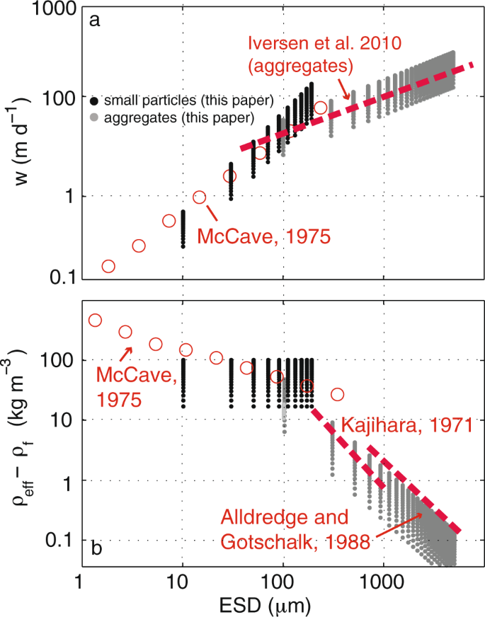
(a) Initial modeled particle sinking velocity (m d⁻¹) and (b) excess density (ρ_eff − ρ_T) as a function of size (equivalent spherical diameter ESD) for small particles (ρ_p = ρ_eff, black points) and aggregates (gray points) at t=0 released at the base of the euphotic zone. The fluid density ρ_T = 1028 kg m⁻³ and α ranges from 0.01 to 0.1. A fractal dimension of 1.85 and A_f = 1.49³⁸ reproduces the flattened w spectrum observed in situ for larger, fluffier aggregates (red dashed lines) with less excess density^27,39,40.

Full size image

Aggregates

For large particles, numerous observations of settling rate versus size demonstrate that the spectrum is flatter than that predicted by Stokes’ equation applied to spherical particles^9,27. Abundant observations from in situ cameras¹⁹, laser imaging⁴¹, SCUBA divers⁴⁰, and gel traps indicate much of the particle mass in the twilight zone is composed of ‘marine snow’, aggregates, or clumps of smaller particles that form ‘fluffy’ particles up to 5 ~ mm²⁷. Compared to a solid particle of similar size and shape, the reduction in the effective density of these porous particles decreases the gravitational force and results in sinking rates that are lower. Applying fractal scaling concepts³⁸ to describe the particles, and using the same procedure as above (see Supplementary Sec. 2 for a full derivation), we can calculate the mass flux of aggregates as

({rm{where}})

D is the fractal dimension (1.6 < D < 3³⁸), A_f is a constant³⁸ and a_s is the sub-particle radius (Supplementary Fig. S2). It is satisfying to note that the aggregate solution converges to that for a solid particle (eqn 9) as D approaches 3 (the fractal dimension of a solid sphere) and as a_s approaches a₀.

Numerous observations of settling rate versus size demonstrate that (particularly for larger aggregate particles) the spectra are flatter than predicted by Stokes’ equation applied to spherical particles^9,27. In our model, the spectrum flattens as the fractal dimension D is reduced below that predicted for a solid particle (D < 3). Here, a fractal dimension of D = 1.85 optimizes the fit between the theoretical settling rate (gray points, Fig. 3a) and the relationship observed²⁷ for large aggregates (red dashed line). The modeled sinking rate at z = 0 with α ranging from 0.01 to 0.1 for small particles (spread in the black points, Fig. 3a) spans a similar range to what is observed (red circles)²⁹.

Laboratory-based studies indicate that typical sinking speeds of individual diatom cells range from 0.1–10 m d^−1 42, and aggregates sink at 88–569 m d⁻¹²⁷. Using optical proxies, silica-depleted diatom cysts⁴³ were observed to be sinking at 75 m d⁻¹ during the North Atlantic spring bloom⁴⁴. Plumes of aggregates (>1 mm) were found to be sinking at 45–108 m d⁻¹ in the California Current⁴⁵. The size-specific settling rate near the west Antarctica Peninsula³⁷ showed large departures from the monotonic increase in settling predicted by Stokes’, potentially due to size-dependent density or shape characteristics.

The excess density of oceanic particles is challenging to measure directly and has generally been inferred from the Stokes’ equation using the sinking velocity, size, and fluid density^29,39,40,46. McCave (1975)²⁹ quantified the sinking rate of small organic particulates from various ocean basins over the size (diameter) range of 1.4 to 362 μm (open circles, Fig. 3a). The sinking rates for these particles ranged from 0.1 to 100 m d⁻¹, from which, a excess density ranging between 500 and 29 kg m⁻³ was inferred (open circles, Fig. 3a). Eppley⁴⁷ performed similar tests on living and senescent diatoms, finding an enhanced excess density (and higher sinking rate) for the latter category. In our model, solid particles have a size-independent excess density (black points, Fig. 3b) that has a similar magnitude to the observed values²⁹. However, a weakly negative relationship observed between excess density and size²⁹ suggests that even small particles may have aggregate-like characteristics⁴⁸. Observations of large aggregates^39,40 revealed a negatively sloped excess density spectrum (red dashed lines, Fig. 3b) up to two orders of magnitude lower than that predicted for smaller particles (red dashed lines, Fig. 3b). Similarly, the model predicts a negative slope for aggregates, as the volume fraction of particulate material decreases as aggregate size increases.

Particle compressibility

In a stable water column, the absolute density of seawater increases by roughly 6% between the base of the euphotic zone and 1000 m depth, as a result of increasing hydrostatic pressure. In comparison, variation in temperature and salinity with depth cause an increase in density of only 1% to 2% (depending on season and region). For organic marine particles that are only marginally denser than the ambient seawater, variations in the density of seawater have a potentially significant impact on the depth to which a particle will sink. The importance of depth-dependent variations of ρ_f depend, to first order, upon the compressibility of the particles themselves. For incompressible particles, we recommend using a value of β that is based on a linear fit between the seawater’s absolute density and depth (see Fig. 4a), whereas for compressible particles, a fit based on potential density may be most appropriate (see Fig. 4b). Overall, we find that most dense particles with (α > 0.01) will not strongly ‘feel’ the effect of density, whereas those that have a small α may be strongly affected, reaching a suspension depth before being remineralized. In Fig. 5 we illustrate the different fates for an incompressible and compressible particle with a density only slightly greater (α = 0.0004) than the density at the base of the euphotic zone (ρ_T). In this case, the incompressible particle will reach a neutral density at a much shallower depth (thick black line, Fig. 5) than the depth reached by particles with a similar compressibility as seawater (thin black line, Fig. 5).

Figure 4

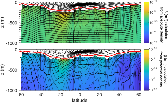
Meridional transects of β reflecting (a) pressure-driven absolute density, and (b) potential density. These values were computed from the WOA09 database from zonal averages between 10.5 to 28.5 ^oW in the Atlantic Ocean. Thick black lines indicate the density contours, and the red line is the mean euphotic depth from a climatological SeaWIFS K490 product. β is calculated over over the depth range examined in our model from z_eu to 1000 m.

Full size image

Figure 5

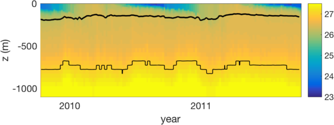
Time-series of potential density -1000 kg m^-3 (σ_t, colors) from ARGO float 6391bermuda (from the chemical sensor group at MBARI www.mbari.org) with contour lines indicating the depth of neutral density for a compressible (thick line) and incompressible (thin line) particle with density ρ_p = 1027 kg m⁻³.

Full size image

Functional form of particle remineralization

The generalized form for particle volume loss (remineralization) is given in equation (2), wherein the value of n determines whether remineralization occurs (a) at a constant rate (n = 0), suggesting that a fixed number of bacteria colonize the particle irrespective of particle size, (b) proportional to the surface area (n = 2), or (c) proportional to the particle volume (or mass) (n = 3). To be dimensionally consistent, the constant C_n takes the form ({C}_{0}={a}_{o}^{3}/3), C₂ = a_o and C₃ = 3 for n = 0, 2, 3, respectively. Here, magnitudes for C and r were selected to produce an overall life-span of about 10 days (Fig. 6a). These three cases produce markedly different behavior over time: particle size (a) diminishes linearly for n = 2 (solid black line Fig. 6a), at an increasing rate with constant remineralization (n = 0, dashed line Fig. 6a), and at a slowing rate with n = 3 (gray line Fig. 6a). Since sinking speed is proportional to a², it means that although the life-span of each particle case is similar, particles that are initially consumed more rapidly (n = 3) do not sink as deep as particles that that are consumed steadily (n = 2) (Fig. 6b). Thus, while the overall shape of the flux profile retains a Martin-like shape (Fig. 6c), it appears that the functional form of remineralization actually impacts the efficiency of transfer.

Figure 6

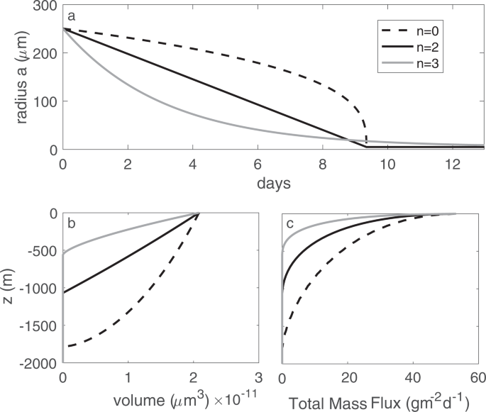
(a) The change in size of a particle of initial radius a_o,i = 250 μm, r = 0.11 d⁻¹, as it is consumed according to eqn (2) for the three remineralization cases n = 0, n = 2 and n = 3. (b) The change in volume as a function of depth for a single size class of particles with a_o,i = 250 μm. (c) The resulting flux profile obtained from integrating over a range of size classes with a size spectral slope of −3, as in Fig. 2.

Full size image

Sensitivity of the flux profile to particle density, slope of the particle size spectrum, remineralization rate and oceanic density stratification

To assess the sensitivity of the modeled flux profile to our remaining parameters: particle density (α), size spectral slope (p) and remineralization rate (r), we generated 27 flux profiles for which we vary one parameter while holding the others constant. For each profile, we quantify the transfer efficiency, T₁₀₀, the ratio of the mass flux at the base of the euphotic zone (z = 0) to the mass flux 100 m below the euphotic zone (z = 100m)⁵⁰

shown with open circles connected by a dashed line in Fig. 7. The range of parameter values were selected from published field and laboratory observations (Table 1), and produce a variety of flux profile shapes and efficiencies (Fig. 7). We fit (fit) each of the modeled (mod) curves (by minimizing the rms error) with a power law (Martin curve) fit F(z) = F(100m) (z /100m)^b and an exponential fit F(z) = F(0m) exp(− z/z^*). The mean rms error is defined as

We find that 11 (of 27) cases modeled are better fit by an exponential, 10 are better fit by a power law, and for the remaining 6, neither the exponential nor power law fit is distinguishably better. Essentially, neither a power law nor exponential form is clearly better at describing these profiles. We had hoped that in performing this test, we could shed light or which is the more suitable form to use for empirical data fitting, but the answer remains elusive. In the following sections, we examine the role that each of the model parameters plays in shaping this curve.

Figure 7

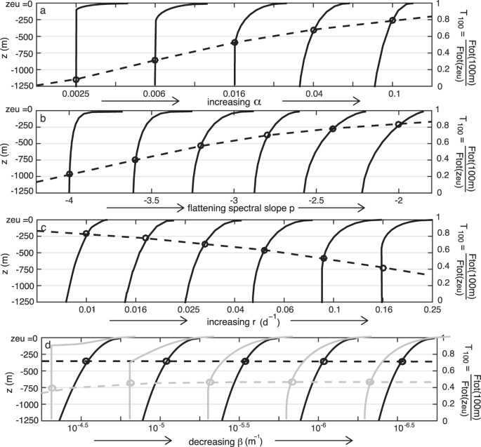
Variety of flux profiles (solid lines) that are obtained from Equations 10 and 11 spanning the observed ranges of (a) excess particle density factor α, (b) initial size spectral slope p, (c) remineralization rate r and (d) vertical density change β. In each case, one parameter is varied, and the others are kept fixed at α = 0.03, p = − 3, r = 0.05 d⁻¹ and β = 5 × 10⁻⁶ m⁻¹ (black lines). For panel (d) we overlay (in gray) flux profiles obtained with α = 0.005 to demonstrate that the profiles are sensitive to β when α is very small. The transfer efficiency T₁₀₀ is shown with open circles intersecting each profile, with its magnitude defined by the axis on the right hand side of the plots.

Full size image

Particle density

The excess density of oceanic particles is challenging to measure directly and has typically been inferred from the Stokes’ equation using the sinking velocity, size, and fluid density^29,39,40,46. McCave (1975)²⁹ quantified the sinking rate of small organic particulates from various ocean basins over the size (diameter) range of 1.4 to 362 μm. The sinking rates for these particles ranged from 0.1 to 100 m d⁻¹, from which, an excess density ranging between 500 and 29 kg m⁻³ was inferred. Eppley et al.⁴⁷ performed similar tests on living and senescent diatoms, finding an enhanced excess density (and higher sinking rate) for the latter category.

As anticipated, increasing the excess particle density factor α results in an increased efficiency of export (open circles, Fig. 7a), as denser particles sink faster, are less affected by changes in the ambient fluid density β, and reach greater depths before they are remineralized. A similar result was obtained by Cram et al.¹³ for a larger percentage of ballast in particles. Over the modeled range of α = (0.002–0.1), between 8% and 80% of the exported material escapes consumption within z = 100 m according to the model.

Slope of the particle size spectrum

Flattening the initial size spectrum of a_o,i and transitioning the mass spectrum from one dominated by small particles (p < −3) to one dominated by large particles (p > −3) also increases the transfer efficiency (Fig. 7b) as in Cram et al.¹³. Under our assumption that particles are remineralized at a steady rate, this makes intuitive sense. As with increasing α, larger particles sink more rapidly and reach greater depths before they are remineralized. The model predicts that T₁₀₀ could vary between 0.2 and 0.84 for variations in p between −4 and −2 throughout the global ocean¹⁹.

Remineralization rate

As predicted in other export models⁵¹, we find that increasing remineralization rate over a range of observed values (r = 0.01–0.16 d⁻¹) attenuates the flux profile and decreases the export efficiency T₁₀₀ from 0.82 to 0.4 (Fig. 7c). We also find that the functional form selected for r (equation 2) can alter the depth to which a particle is likely to sink (Fig. 6b) and transfer efficiency (Fig. 6c). In the Discussion, we evaluate the different circumstances under which one might choose a particular functional form over another. A model that explicitly includes a temperature-dependent^13,28,52 or oxygen-dependant¹³r could allow more material to sink to depth than is predicted by our model. Additionally, variability in r may arise from losses and transformations of POC through zooplankton feeding and egestion^53,54,55 and from the varied composition of particles.

Water column density change

As a particle sinks it encounters denser water, the relative density between water and particle is reduced, the buoyancy force on the particle increases, and the particle may slow down or become suspended. While the effect of density stratification on sinking marine snow or pellets has been considered in other literature^56,57, mechanistic flux models^10,12,13 have not included vertical density changes. The parameter β approximates the linear change in water column density with depth according to (4). Since this parameter is not reported in previous literature, we calculate it explicitly from World Ocean Atlas data across a meridional transect between the climatological euphotic depth (red line, Fig. 4) and 1000 m. We consider β calculated from the absolute density (Fig. 4a), as would be appropriate for incompressible particles (see the earlier section on ‘Particle compressibility’), and β calculated from the potential density (Fig. 4b), as appropriate for compressible particles. Across this transect, β varies from about 5 × 10⁻⁴ to 5 × 10⁻⁶. The effect of β is pronounced for particle densities that are only slightly greater than ρ_T (i.e. α = 0.005, gray lines Fig. 7d). However, for perhaps a more typical value of α = 0.03, the overall flux profile is not very sensitive to the choice of β (Fig. 7d). Interestingly, for the low α case, though the overall profile shape (solid gray lines) is strongly altered by β, this sensitivity is not reflected in the transfer efficiency, which remains between 0.4 and 0.5 for each of the five cases considered (dashed gray line). This is because β has the largest impact when the particles reach a suspension depth (as is the case for the first two gray profiles, β = 10^−4.5 and 10⁻⁵ m⁻¹ on Fig. 7d), but does not appear to strongly alter the shape of the profile above that depth.

Evolution of the particle size spectrum with depth

The model described here, as well as the models of Kriest and Oschiles¹² and De Vries et al.¹⁰, predict that the size spectrum of particles will flatten with increasing depth in the water column, as smaller particles are lost through remineralization and not replenished in large enough numbers by the remineralization of larger particles, of which there are relatively few (Supplementary Sec. 1). However, there is no hint of such a flattening of size spectra in observational data¹⁹. Several reasons can be postulated for this: (i) A large particle undergoes disaggregation or break up into many smaller particles during its descent; (ii) Particles contain hard, mineralogical or recalcitrant bits, so that the remineralization rate diminishes with particle size as the softer material is eaten away; (iii) the net particle density increases with diminishing particle size for the same reason. While a disaggregation model is beyond the scope of this study, we show that by decreasing particle density (Fig. 8) or increasing r (not shown) with particle size, the slope of the size spectrum can be largely maintained with depth. Fig. (8a) provides a demonstration of how size spectra may be altered with depth as a result of a linear dependence between α and size. The range in α selected here is based on the observed ranges cited in Table 1, and the hypothesis that small particles are likely to be more dense (with more ballast) than their larger, more fluffy counterparts¹⁷. This approach provides a plausible remedy to the inconsistency of our original model, as well as other models^10,12.

Figure 8

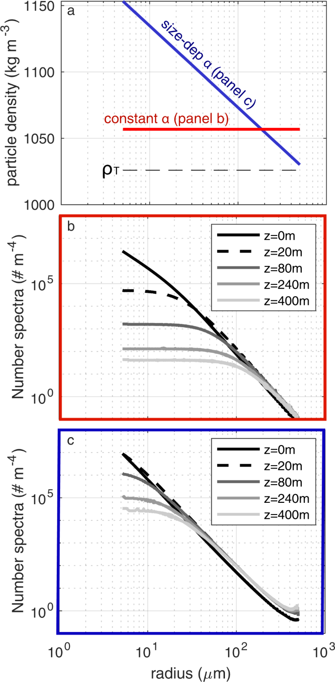
A size-dependant particle density can be used to counteract the flattening effect seen with depth in the model. (a) The excess density that results from a constant α = 0.03 (blue line) and α that linearly decreases from 0.125 to 0.004 over the specified log-distribution of particle sizes (red line). (b) The size spectrum is shown to flatten with depth in the constant α case. (c) With a size-dependant α, this effect is markedly reduced. A similar result can be achieved with an r that increases with increasing particle size (not shown).

Full size image

Modeling a transient phytoplankton bloom by varying the particle size spectrum

A transient phytoplankton bloom is simulated by steepening the size-spectral slope from p = −2 to p = −4.5 over 3 days to represent the transition from early bloom, with production of more large particles (diatoms) to late bloom, which is dominated by smaller particles. Such a scenario was observed during the North Atlantic Bloom experiment, where diatoms dominated the early bloom, but were superseded by smaller phytoplankton when silica ran out^44,58.

For the transient solution, we are no longer able to use the analytic solution and, instead, implement the model numerically. Initially, the slope of the particle size spectrum is set to p = −2. The model is integrated for 16 days until the solution reaches a steady state. From day 16–19, the size-spectral slope is changed linearly from p = −2 to p = − 4.5. After day 19, p is held constant until the new steady state is reached. As p is varied, the total mass flux leaving the base of the euphotic zone is held constant. This ensures that only the relative numbers of large and small particles are varied without introducing changes to the total mass flux entering the water column.

Numerical model

We use a Lagrangian model based on Jokulsdottir and Archer¹¹ to compute the time-dependent solution. A particle object is used to represent a certain number of particles with identical properties, such as size and density, when released from the base of the euphotic layer. Particle objects can be created at each time step, and their trajectories are found by numerically integrating Equation (5) using the Forward Euler method and interpolating the solution onto a grid with 0.5 m resolution. A time step of 1 hour yields a percent error <0.4% when comparing the analytical and numerical solutions for a 250 μm particle, sinking over the course of 20 days. The mass flux at each time is calculated as F_m(t) = N₀ρ_pV(t) where (V(t)=frac{4}{3}pi {[{a}_{0}(1-rt)]}^{3}) for the remineralization case n = 2. The total mass flux is a function of depth and time and is obtained by summing all the particle objects. For the transient bloom simulation, ten particle objects are created at each time step with size classes ranging from 25 to 250 μm. The values of α = 0.03, r = 0.05 d⁻¹, and β = 5 × 10⁻⁶ m⁻¹ are used for all particle objects.

Results of numerical model

Figure 9 shows the total mass flux profiles at four different times of the simulated transient bloom. The profile on day 16 (dashed line) is the initial steady state profile for p = −2, which represents a relative abundance of large particles. The final steady state profile for p = −4.5 corresponding to a relative abundance of small particles is reached by day 32 (light gray line). Profiles between days 16 and 32 show the transition between these two steady states as a result of varying the size-spectral slope at the base of the euphotic layer from day 16 to 19. A subsurface mass flux peak is seen in Fig. 9 on day 19 (black solid line) at a depth of z = 500 m. This subsurface bump then propagates down through the water column with time, reaching a depth of around z = 1250 m by day 22 (dark gray curve in Fig. 9). Note that the total mass flux entering the water column is held constant, so these subsurface peaks are solely the result of changing p at z = 0 m.

Figure 9

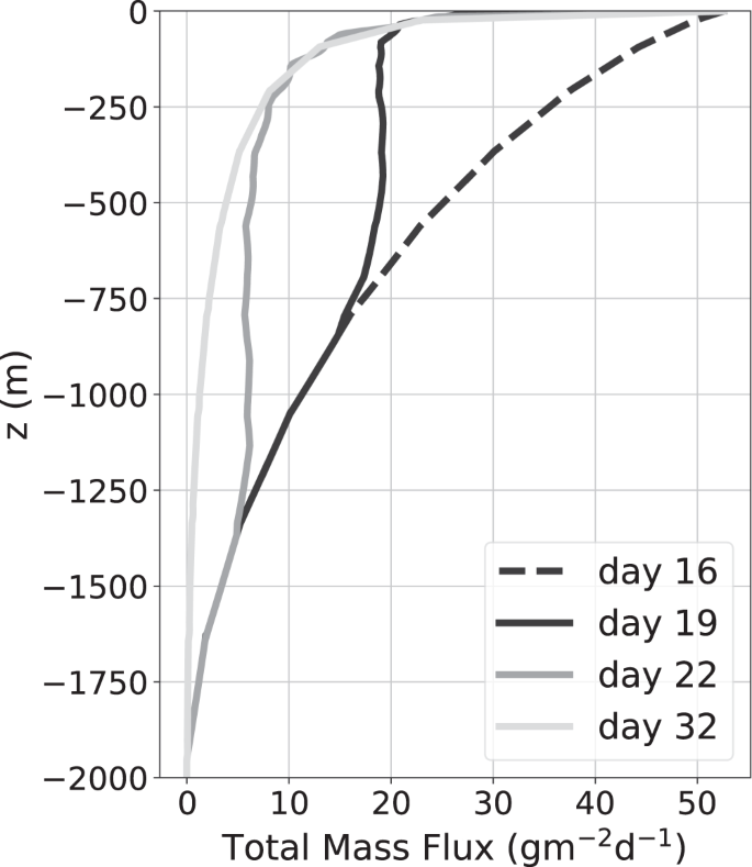
Time evolution of the vertical flux profile as the slope of the particle size spectrum is varied linearly in time from p = −2 on day 16 to p = −4.5 on day 19, after which it is held constant. The total mass flux exiting the euphotic layer is held constant and other parameters are fixed at α = 0.03, r = 0.05 d⁻¹, and β = 5 × 10⁻⁶ m⁻¹.

Full size image

The particle size spectra (PSD) at a depth of 500 m (Fig. 10) reveal that the bump in the flux profile (Fig. 9) is caused by a relative abundance of large particles compared to small particles at the base of the euphotic layer. On day 19, the size spectrum at z = 0 m is steepened so there is a reduction in the number of large particles entering the water column. However, it takes time for this information to reach depth, so the size spectrum at z = 500 m is still relatively flat, and there are more larger particles at z = 500 m than at z = 0 m on day 19. This excess of large particles at depth creates the subsurface maxima in mass flux seen in Fig. 9. Similarly on day 22, the excess of large particles at z = 1250 m results in another subsurface maxima in mass flux.

Figure 10

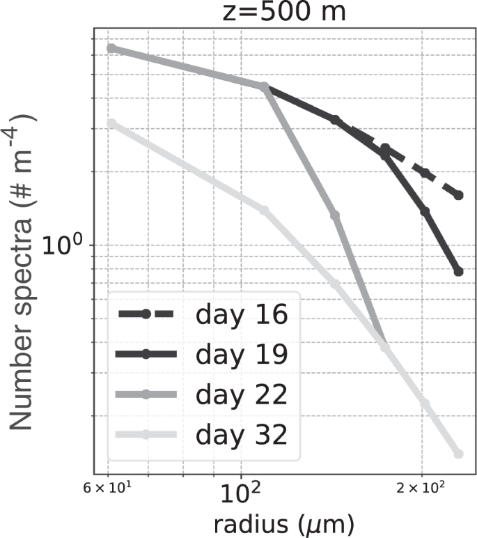
Time-evolution of the particle size spectrum (PSD) at z = 500 m as the number spectral slope at the surface was varied from p = −2 to p = −4.5. The largest particles transition more rapidly to the new steady-state, and the smallest particles transition more slowly.

Full size image

Furthermore, the numerical model reveals how the transition between two steady states occurs. Because larger particles sink faster in this model, the transition between two steady-state spectra occurs starting with the largest particles. For example, Fig. 10 shows the time-evolution of the size spectrum at z = 500 m. As p is steepened at z = 0 m, the spectrum at z = 500 m steepens starting from the largest particle sizes. By day 22, the largest three particle sizes have already reached the new steady-state spectrum. In contrast, the smaller particles do not reach the new steady-state spectrum until day 32. This is because the small particles sink more slowly, so it takes longer for information about changes in small particles at the surface to reach depth.

Source: Ecology - nature.com