Ethics approval and consent to participate
The research permits, including the appropriate ethic approvals, were obtained for this study from the CNERSH (Comité national d’Ethique de la Recherche pour la Santé Humaine) in Cameroon (Approval N°2017/05/900), as well as from regional health districts (Centre region, Approval N°0061). We further obtained an ethical approval from the French CPP (Comité de Protection des Personnes, approval N°2016-sept-14344), as well as the authorization to import and store these samples from the French Ministry of Higher Education and Research (N°IE-2016-876 and DC-2016-2740, respectively). Finally, we obtained the authorization to store personal data in France from the CNIL (Commission Nationale Informatique et Libertés, N°1972648). We obtained the informed consent of each participant for contributing to this research and publishing the associated-data. Consent for publication is not applicable. All research was performed in accordance with relevant guidelines and regulations.
Sampling and collection of contextual data
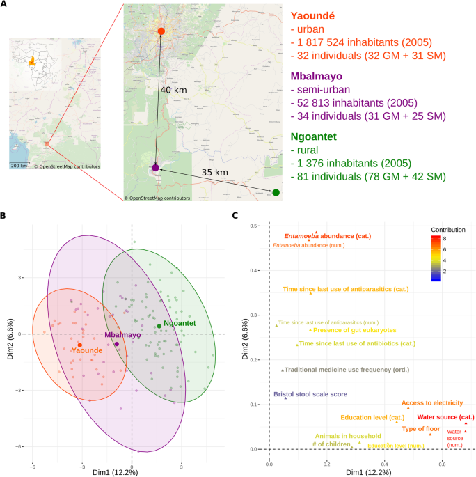
We sampled 147 adult volunteers at three locations in Cameroon (Fig. 1A), representing an urbanization gradient: 81 individuals in Ngoantet (rural), 34 in Mbalmayo (semi-urban) and 32 in Yaoundé (urban), after obtaining their informed consent. The participants declared being currently healthy, i.e. not taking medication for any infectious or metabolic disease or suffering from specific symptoms (e.g. fever). They were between 18 and 65 years old and were not related at the second degree. They self-collected the feces during the morning in sterile recipients provided by us (Medline stool containers). We then placed app. 3 g of the fecal samples into 60 mL containers with RNAlater. For saliva, the participants spit 2 mL of saliva into a 15 mL falcon tube, to which we added the same volume of a homemade buffer (5 mM TRIS, 5 mM EDTA, 5 mM sucrose, 10 mM NaCl, 1% SDS, pH = 8).
In addition, we recorded contextual information (metadata) about the participants (Supplementary Table 1) in collaboration with local investigators and trained research assistants. Specifically, we collected dietary information using a quantitative 24-hour recall questionnaire (recording the amount of all the items the individual has eaten during the last 24 hours, which is then transformed into the amounts of nutrients and energy ingested) and a qualitative food frequency questionnaire (FFQ, reporting how often the selected types of food were consumed during the last month50). The FFQ data were collected only for the rural and urban population. Non-dietary information including medical (use of antibiotics, antiparasitics, and traditional medicine) and other socio-economic and socio-demographic variables (water source, type of floor, animals in household, access to electricity, smoking, number of children, education) were collected using questionnaires. Only the animals that were declared by the participants to live in the house were considered as the animals in the household and included: cats, dogs, guinea pigs, parrots, goats, pigs, ducks and poultry. We did not consider the presence of mice. For smoking habits, we grouped individuals into five groups: non-smokers (“0_non”), “1_recent”, who started smoking during the last year, “2_medium”, who have smoked for less than 5 years, “3_longtime” – smoking for 5+ years, less than 10 times a day and “4_longtimeHeavy” – smoking for 5+ years, 10 or more times a day.
Anthropometric traits (height and weight) were measured using standardized techniques. The Centre Pasteur du Cameroun furthermore performed a microscopic analysis of the fecal samples to identify the gut eukaryotes (with a bias toward the identification of potentially pathogenic species, i.e., worms and Entamoeba sp.). For Entamoeba sp., we grouped individuals in categories depending on the output of the microscopic analysis as follows: “0_ none” if no cyst nor any trophozoites was seen; “1_rare” if only rare cysts were observed; “2_some” if only few cysts or few trophozoites were observed; “3_abundant” if numerous cysts and/or trophozoites were observed. Finally, we estimated the Bristol stool scale score by visually assessing the stool consistency (a proxy for colonic transit time and water content51).
DNA extraction and sequencing
App. 250 mg of fecal material was disrupted by bead-beating and DNA was subsequently extracted with the MOBIO PowerFecal DNA isolation kit (MOBIO Laboratories, Carlsbad, CA, USA) according to the manufacturer’s protocol. DNA from the saliva samples was extracted following the protocol of Quinque et al.52. The extracted DNA was quantified with NanoDrop (ThermoScientific). Sequencing libraries targeting the V4 region of the 16S rRNA gene were prepared by the MOC core facility at the Broad Institute, Cambridge, MA, USA and sequenced as 150 bp paired-end reads in two runs on an Illumina MiSeq. 300 (as described in53), resulting in an average of 61,617 ± 43,997 (st. dev.) raw reads per sample (Supplementary Table 9).
Data analysis
All analyses were performed in R54 except for the parts of sequencing data preprocessing that was done in mothur55.
Metadata analysis
We imputed missing values in the contextual data using the missForest R package56. In order to assess the strength of pairwise correlations between the variables, we calculated Pearson’s r for pairs of numerical variables, Cramer’s V for categorical predictors (using the rcompanion package57 and omega for numerical-categorical combinations. We disregarded all correlation coefficients for which the t-test, chi-square test or Kruskal-Wallis test (for numerical, categorical and numerical-categorical variables, respectively) were not significant at alpha = 0.05. In addition to the urbanization level variable, we analyzed 51 variables collected in all three populations: 28 dietary variables from a 24h-recall questionnaire and 23 non-dietary variables. We analyzed 49 additional dietary FFQ variables for the urban and rural populations only. The presence of Entamoeba sp. and smoking habits were encoded both as binary, as well as ordered factors (specifying Entamoeba sp. load and smoking intensity and duration), which resulted in a total of 25 non-dietary variables tested for correlations. After correcting for multiple testing, 403 out of 1431 (28%) and 555 out of 5253 (11%) pairwise correlations between these variables were significant in the complete and rural-urban dataset, respectively (alpha = 0.05, Supplementary Table 4). Strong correlations (abs(Pearson) >= 0.8, Cramer’s V or Omega >= 0.4) were mainly found between 24h-recall dietary variables and between habitat-related (e.g. sanitary) variables (Supplementary Fig. 1). In addition, the urbanization level was associated with some habitat-related variables, including water source, access to electricity, type of floor and presence of animals in the house. The inclusion of the dietary FFQ data (and omission of semi-urban samples) revealed some additional correlations, notably between the urbanization level (or some of the associated habitat-related variables) and: education level, number of children and consumption of meat, cassava and peanuts.
In order to explore the multivariate aspects of the contextual data and to identify the factors that best describe the urbanization gradient, we used the FactoMineR package58. We first performed a factor analysis of mixed data (FAMD) with all non-dietary variables. The categorical variables representing the ordered factors were duplicated and one version was coded as a numerical while the other was coded as a categorical variable. We performed a separate PCA on 24h-recall dietary data normalized by total energy input, as well as on the FFQ data for the rural-urban data subset only. In each case, the correlation coefficient between the ordination axes and urbanization level were calculated with dimdesc in order to statistically test the representation of the urbanization gradient by the axes. In addition, we tested the association between FFQ data and urbanization level with the v test from the same package (function “catdes”).
Sequencing data quality control, taxonomy assignment and OTU clustering
Sequences were denoised using dada259 according to the authors’ recommendations. First, the reads were processed with the filterAndTrim command in order to remove phiX spike-in and reads with ambiguous bases, to truncate reads at the first base with quality score <= 2 and to filter reads with more than 2 expected errors. The sequences were then dereplicated with the derepFastq function. Subsequently, the error rate was estimated from a subset of 1,000,000 reads for each run separately using the learnErrors function. These error rate estimates were used in the actual denoising function, dada, run with the option pool = T. The denoised forward and reverse reads were merged with mergePairs command in order to obtain amplicon sequence variants (ASVs). Finally, we created input files for further processing in mothur55: a fasta file and a group file (assigning sequences to samples). In summary, 83% (12 800 410/15 398 557) of raw reads passed quality control and denoising steps (Supplementary Table 9). We removed 11 out of 250 samples due to low number of reads (<1500). The remaining 239 (141 fecal and 98 saliva) samples contained on average 53 540 reads (±34 540).
We used mothur to assign taxonomy, remove non-bacterial sequences and cluster OTUs, following the MiSeq standard operating procedure60. Briefly, we classified sequences with mothur implementation of RDP classifier61 using the RDP Release 11 taxonomy62 with 80% confidence cutoff and filtered out unclassified and non-bacterial sequences. We aligned the sequences to the V4 region of the SILVA v132 reference alignment63 and removed the chimeras with CATCh64. We used OptiClust65 with Matthews correlation coefficient (MCC) optimization to create 85–99%ID OTUs at 0.01 steps and applied 80% confidence cutoff for the consensus OTU taxonomy. OTU representative sequences were defined as the sequences with the smallest average distance to all the other sequences within a given OTU.
In order to explore the effect of OTU clustering method, we used also another, phylogeny-based approach, bdtt66, which creates the OTUs by slicing of a phylogenetic tree (whose construction is described below) at a specified evolutionary distance. We sliced the tree in the range 0.01–0.15 branch length at 0.01 steps. We modified the original bdtt script in order to add the new, sliced tree and the OTU table to the output. The consensus taxonomy was found as the lowest common ancestor of all sequences within an OTU.
The number of reads and ASVs per sample before and after quality control are reported in Supplementary Table 9. The number of reads and OTUs before and after filtering for each combination of clustering method and cutoff are listed in Supplementary Table 10. We identified in total 4,078 ASVs (grouped into 246 genera), 2,977 of which were found in the fecal microbiome (209 genera) and 2,025 in the saliva microbiome (198 genera).
Phylogenetic tree
The phylogenetic tree was created with RaxML67 following the protocol described in Stamatakis68. We imposed the monophyly of the classes within Proteobacteria on the tree topology as described in Groussin et al.66. We ran 100 independent fast tree searches with GTRGAMMA model, performed a bootstrap analysis (with autoMRE option, which automatically determines how many replicates are needed to get stable support values, in this case 550 trees) on the best tree and created a MR consensus tree. All independent trees were unique and the tree diversity was high (average Robinson-Foulds topology distance = 0.5029), indicating an unstable topology. This was further supported by low relative tree certainty from the bootstrap analysis (0.150089). Still, the best tree was significantly better than the suboptimal ones according to the Shimodaira-Hasegawa test69. Although the results of phylofactorization differed somewhat depending on the tree (not shown), they were overall congruent, so we used the best tree in all analyses (phylogenetic diversity, bdtt OTU clustering and phylofactorization).
Alpha diversity estimates
We calculated rarefactions curves for Good’s coverage and non-phylogenetic alpha diversity indices (observed species, Shannon’S H, inverse Simpson and Berger-Parker dominance) with 1000 iterations at 1000 sequence steps in mothur55. Based on the rarefaction results (not shown), we chose a subsampling depth of 6500 reads per sample for calculating the average (200 replicates) of the above alpha diversity indices. We then transformed these values into the effective number of species as described in Jost70. Effective number of species is the number of species in a perfectly even community that results in a given value of a diversity index. Diversity indices within this framework are mathematically defined as Hill numbers of different order (q) and can be linked to the more traditionally used richness and dominance/evenness indices. The order, q, defines how much weight is given to the abundant species: q = 0 ignores the abundance altogether (and is equal to species richness), q = 1 weighs the species exactly according to their abundance (and corresponds to exp(Shannon’s H)), q = 2 is the same as inverse Simpson index and gives emphasis to dominant species, whereas q = Inf corresponds to the inverse of Berger-Parker dominance, and thus depends only on the relative abundance of the most abundant species. The advantage of these indices is that they are intuitive and easily interpretable: they have common units and possess doubling property (i.e. diversity of a union of two communities with completely distinct species is the sum of diversities of the two component communities). Jost70 refers to these diversity indices as “diversity of order 0, 1, 2”. We use here their mathematical denotations – 0D, 1D, 2D and InfD – for brevity.
Chao et al.71 developed a corresponding Hill-number framework for phylogenetic diversity. The main idea is the same, but here the diversity is defined as effective number of lineages, corresponding to the phylogenetic diversity of a perfectly even community composed of perfectly distinct species. We used the hillR R package72 to calculate average phylogenetic diversity indices of order 0, 1 and 2 of 20 dataset replicates subsampled to 6500 reads/sample. We refer to these indices as 0Dph, 1Dph, 2Dph..
Filtering for beta diversity analysis and community type determination
In order to get rid of the noise and to reduce the complexity of the dataset, we performed a two-step unsupervised filtering implemented in the PERFect package73. Briefly, the method compares the total covariance of the community data (“OTU table”) before and after removal of a taxon. This “difference in filtering loss” is then compared with a null distribution and the taxon is retained or discarded for a given significance level alpha (here alpha = 0.1). Based on the empirical evidence and authors’ suggestions, we assumed that at least 50% of taxa were not informative and therefore fitted a skew-normal distribution to the observed filtering loss values. In the first step, called simultaneous filtering, the taxa are ordered according to the number of occurrences and filtered sequentially as long as the filtering loss values come from the null distribution; in the second step, called permutation filtering, the taxa are ordered according to the p-values from the first step and filtered based on an additional permutation step (1000 replicates) that ensures that only the taxa that are uninformative for any combination of retained taxa are removed. We filtered the gut and saliva microbiome datasets separately. Filtering for beta diversity analyses resulted in 282 ASVs for the fecal and 110 ASVs for the saliva dataset (Supplementary Tables 9 and 10). This filtering step reduced the number of reads by 31% and 9% in the fecal and saliva datasets respectively, while eliminating on average 90% and 88% of the ASVs/OTUs/genera, regardless of the clustering method and cutoff.
As the compositional methods that we used to statistically analyze the data do not allow zero values, we replaced zeros utilizing the Bayesian multiplicative replacement function (cmult.repl, method = “GBM”) implemented in the zCompositions R package74.
For distance-based analyses, we performed a centered log ratio (clr) transformation75 implemented in the CoDaSeq R package76,77 and calculated the Euclidean distances, corresponding to Aitchison distances of raw compositional data78. For community type determination, we grouped the non-filtered ASV dataset at the genus level with the phyloseq “tax_glom” command79.
Statistical analysis: microbiome diversity and composition along the urbanization gradient
To examine how the human microbiome diversity changes along the urbanization gradient, we analyzed the gut and saliva microbiome separately.
For alpha diversity, we fitted generalized least squares (gls) linear models with the package nlme80, with weights allowing different variances for each population in case of heteroscedasticity, i.e. if the Levene’s test of homogeneity of variance (car package81) was significant at alpha = 0.05.
To identify the taxa (ASVs and OTUs) whose relative abundances differed between the populations, we used the ALDEx2 package76,82. We considered the taxa as differentially abundant only if Benjamini-Hochberg adjusted p-values of both Kruskal-Wallis and glm test were significant (p <= 0.05).
Finally, in order to identify the lineages that most predictably vary along the urbanization gradient regardless of the classification level, we performed a phylofactorization using the phylofactor package83, with a custom objective function (the same gls model as used in the alpha diversity analysis), F-statistic as a criterion for choosing the best edge, and KS test as the stopping function.
Statistical analysis: community types
In order to classify the microbiomes into the optimal number of categories, we performed Dirichlet-multinomial mixture (DMM) modelling84 on the genus-level data with the DirichletMultinomial package85. We chose the optimal number of components based on the Laplace goodness-of-fit of models with one to ten components. We calculated associations between enterotypes (gut community types86) and stomatotypes (saliva community types46), as well as between the community types and urbanization using Fisher’s exact test as in44.
Statistical analysis: factors associated with community diversity and composition
As food-frequency questionnaire (FFQ) data were not available for semi-urban samples, we performed each of the following analyses three times: for all samples without FFQ data, and for rural-urban samples with and without FFQ data.
The metadata that we collected included both numerical and categorical, often correlated variables (Supplementary Table 4 and Fig. 1). As it is often not trivial to decide which of the correlated factors are important (representing a problem for stepwise variable selection) and as we wanted to make as few assumptions about the data as possible (e.g. linearity), we used random forest classification and regression for the prediction of community types and alpha diversity, respectively. Random forest regression/classification identifies the best set of predictors, without assuming any particular relationship between the independent and response variables. We used conditional forest algorithm87 implemented in the partykit package88. We followed the guidelines from48 and calculated conditional variable importance with the party package and cutoff = 0.249 in order to avoid biases due to different scale of predictors and correlations between them. We used the caret package89 to split the dataset into a training (80%) and test (20%) subsets and to find the best value for the “mtry” (i.e. available number of variables for splitting at each node) parameter. We used the minimization of RMSE (root mean square error) as the selection criterion for regression and the maximization of Cohen’s Kappa for classification. We ran ten independent iterations on each dataset to get realistic estimates of the mean and variability of the variable importance and the goodness of fit. As there is no clear cutoff for variable selection based on their importance, we applied several approaches. The most relaxed approach was the inclusion of random variables in the models: the factors with lower mean importance than the random variable with the highest value were considered unimportant. The second approach was to keep all the variables with a mean importance above the 95% quantile of all mean importance values. The final approach was to split the mean importances into two groups by kmeans clustering. In the last two approaches, we discarded all predictors if any of the random variables was in the “important” group. We used both variable importance and goodness-of-fit estimates (including R-squared and variance explained by the model). If the proportion of the variance explained or the model accuracy was low (R-squared < 0.1 or Kappa < 0.3), we did not interpret the results.
We analyzed potential associations between the community composition and the metadata by a distance-based approach inspired by Gloor et al.90 and Falony et al.25. Briefly, we performed a Principal Component Analysis on the equivalents of Aitchison distances with the package vegan91. We found the variables significantly associated with the first three axes of variation using the envfit function. If some of the significant variables were correlated (correlation coefficient >= 0.8, Supplementary Table 3), we selected the one that explained more variation in envfit and discarded the rest. We then used these selected variables as a scope for ordistep (bidirectional) variable selection. Finally, we identified the ASVs (or OTUs) whose coordinates were in the lower 2.5% and the upper 97.5% quantile on the first three PCA axes as well as those with the distances in the 2.5% and the upper 97.5% quantile from the coordinates of the selected environmental variables (calculated with the cdist function from the rdist package92.
Statistical analysis: differences between the gut and saliva microbiome
We investigated a potential correlation between the gut and saliva microbiome diversity within individual using Pearson’s r coefficient, with nonparametric bootstrap 95% confidence intervals calculated with the boot package93,94. In order to determine if the gut and saliva microbiome within an individual share more species than expected by chance, we compared the observed within-individual beta diversity values (both Bray-Curtis and species turnover measure that accounts for the differences in species richness between the samples; the measure varies between 1 for identical communities and 2 for completely distinct communities95) with the null distribution created by shuffling the sample labels 10 000 times. We either used free permutations or allowed permutations only within the population, to account for the differences between them. We calculated the p-values as observed rank/10 001 and the standardized effect size as (observed mean – random mean)/random standard deviation.
Source: Ecology - nature.com
