Study sites
Five sites across three estuaries were selected to span a range of environmental conditions (e.g. sediment mud content, organic matter content, chlorophyll concentrations, and macrofaunal community composition). Three of these sites were in the Whangarei Harbour, one was in the Raglan Harbour, and one was in the Whangateau Harbour (Fig. 1).
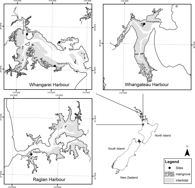
Study sites on the Whangarei, Whangateau, and Raglan Harbours in northern New Zealand.
Whangarei Harbour is a large, unstratified estuary over 20 km long, covering an area of 104 km2 18,19 and with a catchment area of 229 km2 20. Mean depth in the harbour is 4.42 m21, with a mean tidal range of 1.73 m18. Approximately 28% of the harbour flushes each tide, and about half (54 km2) of the harbour area is intertidal20,21. Approximately two thirds of the intertidal area is composed of unvegetated, intertidal flats, with the remainder being mangrove forest and seagrass meadows, both of which have expanded in recent decades22,23. Land use in the catchment varies, with high proportions of pastoral agriculture and plantation forestry alongside urban areas and areas of native vegetation20.
Whangateau Harbour is a shallow estuary of approximately 9.2 km2, with little freshwater input24. The harbour has a high flushing rate, with up to 99% of the water being exchanged with each tide24, and 85% of the harbour is composed of intertidal flats25. The spring tidal range of the harbour is 2.2 m26. The harbour has a small catchment (~ 40 km2 in area), comprised primarily of native forest, but with areas of plantation forestry, livestock agriculture, horticulture, and urban use26.
Raglan Harbour is a drowned river valley of approximately 33 km2 area, of which ~70% is intertidal. The harbour has a maximum depth of 18 m, although channel depths closer to 5 m are more common. Raglan Harbour has a neap tidal range of 1.8 m and a spring tidal range of 2.8 m with 50–75% of the volume of the Harbour being exchanged each tidal cycle (at neap and spring tides respectively). The catchment is large (165 km2), and is dominated by agriculture and plantation forestry which have historically resulted in large inputs of sediment, with small areas of native forest and urban areas27.
Nitrogen enrichment treatments
At each site, three nutrient enrichment treatments were performed: a high N treatment (600 g N m−2), a low N treatment (150 g N m−2), and a control with no enrichment. The application method and treatment doses were based on a previously tested method of nitrogen enrichment in New Zealand intertidal flats, which successfully resulted in long term nitrogen enrichment at treated sites for periods of >6 months28,29. Nitrogen fertiliser was placed in twenty 5 ×15 cm deep cores per m2, using a controlled-release, nitrogen-only, urea fertiliser (with no potassium, phosphorous, or trace elements). Fertiliser was inserted at a depth of 15 cm, with sediment cores removed, fertiliser added, and sediment returned to fill the remainder of the hole created by the core. This enrichment procedure was carried out 6 months prior to GHG flux measurements, in order to avoid impacts of the physical disturbance effects of enrichment and to measure the effect of chronic nutrient enrichment on those fluxes, which have been observed to occur at 3–6 months post nutrient enrichment using the same methodology29.
Each treatment plot was 3 × 3 m in area, and plots were separated by at least 3 m from any other plot within each replicate block (Fig. 2). Treatments were replicated three times at each site in a randomized block design, for a total of nine plots per site. Replicate blocks were situated 10–15 m apart. All plots were located at similar tidal heights (approximately four hours of tidal emergence), with distances in tidal height between treatment plots negligible relative to the tidal range. Measurements carried out using static chambers in Light/Dark pairs separated by 0.2 m within each plot (for a total of 18 benthic chambers per site) and were at least 1 m from plot edges to minimise edge effects across the edge of treatment plots. Chambers were arranged in Light/Dark pairs to capture respiration rates (dark chambers) and the impact of photosynthesis/production (light chambers) on GHG emissions.
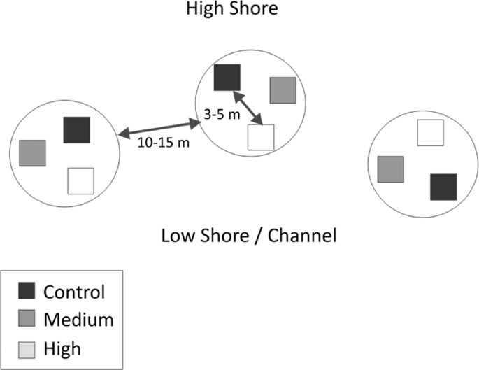
Example site layout of three replicate nutrient enrichment treatments. High Shore and Low Shore/Channel indicate proximity to terrestrial habitats, and toward open water, respectively.
Nutrient enrichment at all sites was performed in April 2017, followed by sampling of GHG fluxes in November and early December 2017. Two of the five sites (Raglan and Whangateau) were re-treated with nitrogen fertiliser in December 2017, and a second round of sampling was carried out at these sites (and in the control treatments of the three sites in Whangarei) in June and July 2018 to investigate seasonal variation in GHG fluxes.
Greenhouse gas flux measurement
GHG fluxes across the sediment-atmospheric interface were measured using 30 L, 0.25 m2 airtight benthic chambers. The measurement chambers were arranged in Light and Dark pairs, with one chamber having a clear lid and one an opaque lid. As soon as the receding tide exposed the study site, chambers were pushed 7 cm into the sediment. After approximately 10 minutes, the lids (and dark covers for dark chambers) were attached and sealed, and 10 minutes after that the first gas sample was taken. The 20 minute period between chamber placement and the start of flux measurements was chosen as a result of a preliminary experiment for this study30. As part of that experiment, the fluxes of GHGs were measured several times throughout the period of emergence at two sites with different environmental conditions, in order to determine the necessary sampling period for this study. The same light/dark paired in situ benthic chamber methods were used as those in this study, but with six gas samples collected from each chamber at approximately 25 minute intervals, instead of only collecting initial and final gas samples. This preliminary experiment showed no evidence of a large initial flux, with the flux of CO2 and CH4 over the first sampling period similar to that in the second and third period for each site, except for the CO2 flux in the light chambers at Onerahi. This provided strong evidence that there was not a high initial flux of GHGs in the chambers resulting from the physical disturbance of placing the chambers in the sediment, as any impact from this disturbance would have been expected across all treatments at all sites. Consequently, a 20-minute delay between the disturbance of placing the chamber and taking the initial measurement was used as a precaution but was considered adequate.
Initial 900 mL gas samples were collected from the chambers within ten minutes of sealing the chambers and stored in Tedlar bags. A final 900 mL gas sample was collected from each chamber immediately prior to tidal submergence at the site. The two samples in combination accounted for approximately 6% of the total 30 L volume of the measurement chamber. The period between the initial and final sampling of gases in the chambers ranged from 2–4 hours in length, depending on the magnitude of the tide, and the presence or absence of wind-driven waves that influenced the duration of tidal emergence/submergence.
Samples were kept in dark, insulated bins at ambient temperature and transported to the University of Auckland laboratory facilities for analysis. Gas samples were analysed within 24 hours of collection, using a Picarro G2508 Gas Analyser to determine the concentration of N2O, CO2, and CH4 gas in the samples. The detection and accuracy limits of the Picarro analyser are listed in the Supplementary Information.
The samples were collected twice for at each site, once in November/December 2017 for all nutrient enrichment treatments, and once in June/July 2018 for all enrichment treatments at the Whangateau and Raglan sites and for the Control treatment at the three sites in Whangarei. More regular sampling was not feasible, in part due to the unavoidable physical disturbance of sampling. It is likely that this disturbance, if it occurred more regularly, would influence the processes at those sites31, altering the fluxes and potentially obscuring the effect of prolonged nutrient enrichment on GHG fluxes.
Flux calculations
Gas concentration measurements from the Picarro Gas Analyser were given in molar parts per million (ppm). To convert this to a standard gas flux (µmol m−2 hr−1), the Ideal Gas Law was used, calculating the molar concentration of a gas at the start and end of the gas sampling and the consequent change over time (Eq. 1).
$$flux=frac{left({G}_{F}times frac{{P}_{F}times V}{Rtimes {T}_{F}}right)-left({G}_{I}times frac{{P}_{I}times V}{Rtimes {T}_{I}}right)}{Atimes Delta t}$$
(1)
where G = concentration of a given GHG in the chamber at the start (I) and end (F) of the measurement (ppm); P = atmospheric pressure at the start (I) and end (F) of the measurement (atmosphere); V = volume of gas in the chamber (L); R = Ideal Gas Constant of 0.0821 L atm mol−1 K−1; T = temperature in the chamber at the start (I) and end (F) of the measurement (K); A = area of sediment covered by chamber (m2); and Δt = time between the start and end of the measurement (hours).
Site characteristics
While there are a multitude of environmental variables that may drive variation in the flux of GHGs, the following variables were selected with the aim of explaining the greatest possible proportion of variation in GHG fluxes with the limited resources available.
Temperature inside the chambers was recorded by 1-Wire i-button DS1921G-F5# automated loggers, located 10 cm from the edge of the chamber and 2 cm above the sediment surface. Photosynthetically Active Radiation (PAR) intensity was measured using two Odyssey Submersible PAR Loggers at each site.
Composite samples of five 2 cm deep, 2.5 cm diameter cores were collected from within 30 cm of the outer edge of each paired light and dark chambers to characterize sediment properties. To calculate pore water content, an approximately 15 g subsample was homogenised, weighed, freeze-dried for 8 days, and weighed again. The difference in weight between samples was calculated, and the proportion of the sample comprised from water expressed as a percentage. Chlorophyll a was analyzed by freeze drying an ~15 g subsample of homogenised sediment, producing approximately 5 g of dry sediment. Samples were boiled in 90% ethanol to extract chlorophyll a32. The extract was processed with a spectrophotometer (Shimadzu UV Spectrophotometer UV-1800). Samples were then acidified to separate phaeophytin from chlorophyll a33. The chlorophyll-a and phaeophytin content of the sediment is an indication of the microphytobenthic biomass that can occur at each site34,35. Due to resource constraints, more comprehensive measures of microbial activity could not be carried out. As such, the chlorophyll-a and phaeophytin content of the sediment are to be used implicitly as proxies for microbial activity.
Organic matter content was estimated using an ~5 g subsample of freeze-dried, homogenized sediment which was weighed, ashed at 450 °C for four hours36, and reweighed. Organic matter was calculated from the difference between dry and ashed weights. While attempts were made to measure the dissolved inorganic nitrogen concentration in the pore water at each site, due to analytical problems that data was unusable. As a result, the organic matter content of the sediment was used as a proxy.
Sediment grain size was measured using a Malvern Mastersizer 3000 (measuring particles 0.1–3500 µm in diameter). Samples were digested in 10% hydrogen peroxide until frothing ceased, rinsed with distilled water in a centrifuge, and run through the Malvern. The mud content was measured as the proportion of grains <63 µm in diameter.
Macrofaunal community characteristics have been found to be important factors influencing the flux of GHGs on temperate intertidal flats, with the abundance of large bioturbating bivalves being key drivers of this influence15,37. Consequently, the macrofaunal community characteristics were sampled once in summer and once in winter for each pair of Light/Dark chambers, using one 15 cm deep, 13 cm diameter sediment core immediately adjacent to the paired chambers (within the treatment plot). Cores were sieved on a 500 µm mesh. For the samples collected during summer, the material retained was preserved in 50% isopropyl alcohol and stained with Rose Bengal for subsequent analysis. All macrofaunal organisms observed were counted and identified to the lowest taxonomic level possible – in most cases species. Macrofaunal sampling in winter was limited to counts and measurements of bivalves >5 mm diameter (Austrovenus stutchburyi, Macomona liliana, and Paphies australis); material was returned to the sampling site.
Statistical analysis
The PERMANOVA + package for PRIMER v7 was used to quantify differences in the environmental variables measured at different sites and in different seasons, and to quantify differences in the flux of GHGs between and within sites, nutrient treatments, light exposure (i.e. Light or Dark chambers), and seasons.
Permanovas were carried out on Euclidian Distance Resemblance matrices, using the fixed factors of Site (Onerahi, Parua Bay, Takahiwai, Raglan, and Whangateau), Treatment (Control, Medium, or High nutrient enrichment), Light Exposure (Light or Dark), and Season (Summer or Winter) for the GHG fluxes.
For environmental variables, the factors of Site and Season were used. The highest order interaction that was significant at the p < 0.05 level was used to analyse differences in flux between groups of these factors. After an interaction was identified, post-hoc pairwise tests were carried out to identify which groups within those interactions were significantly different at the p < 0.05 level, and the direction of those differences.
Source: Ecology - nature.com

