Sample retrieval and DNA sequencing
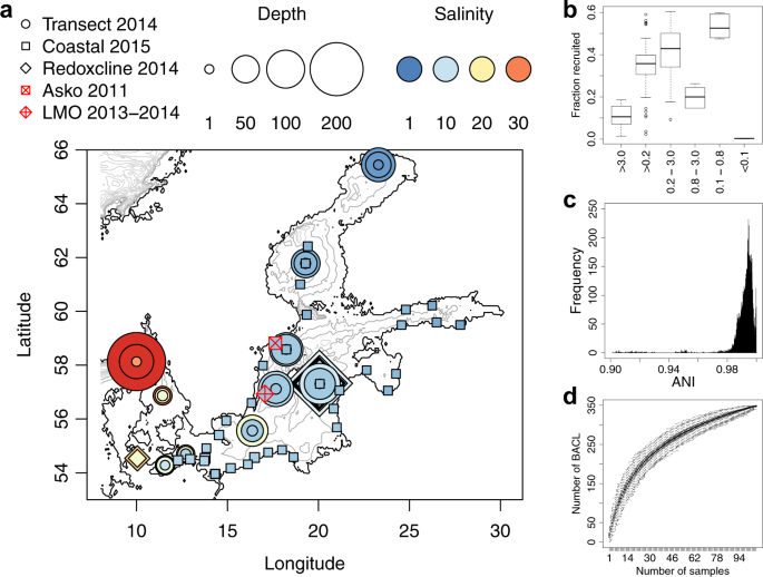
Samples included within this study are divided into five sample sets named Askö Time Series 2011, Redoxcline 2014, Transect 2014, LMO Time Series 2013–2014 and Coastal Transect 2015(Fig. 1a). Metagenome data for three of these have previously been published: Askö Time Series 201160, Redoxcline 201433, Transect 201433; and two are new to this publication: LMO Time Series 2013–2014 and Coastal Transect 2015. For the published sample sets, only a brief description of sample retrieval is given here. For detailed descriptions, the reader is directed to the respective publication.
The Askö Time Series 201160 samples (n = 24) were collected on six occasions between 14 June and 30 August in 2011. On each occasion, the samples were sequentially filtered through 200, 3.0, 0.8 and 0.1 µm filters. DNA was sequenced from the 3.0, 0.8 and 0.1 µm filters, as well from the water passing the 0.1 µm filter.
The Redoxcline 201433 samples (n = 14) target the transition between oxic and anoxic water and were collected on three occasions in 2014, from the Gotland Deep on October 18 (n = 2) and October 26 (n = 8) and from the Boknis Eck61 station on September 23 (n = 4). The October 18 samples were captured on a 0.2 µm filter without pre-filtration while all other samples were filtered either on 3.0 µm filter without pre-filtration (n = 6), or on a 0.2 µm filter using 3.0 µm filter for pre-filtration (n = 6).
The Transect 201433 samples (n = 30) were collected during a cruise in June 2014. Samples were taken from three different depths, spanning the oxygenated zone, at ten stations covering the horizontal salinity gradient. Samples were captured on a 0.2 µm filter without pre-filtration.
The LMO Time Series 2013–2014 samples (n = 22) were collected from the Linnaeus Microbial Observatory station 10 km east of Öland (Latitude 56.938436, Longitude 17.06204) from January 2013 to December 201462. 10 liter samples from surface water (2 m depth) were collected using a Ruttner sampler and transported to the laboratory in carefully acid rinsed polycarbonate containers. 3–5 liter of seawater were filtered through 0.22 µm filters (Sterivex, Millipore) to harvest cells, following pre-filtration through 3.0 µm filters (Poretics polycarbonate, GVS Life Sciences). DNA was extracted using the protocol by Boström et al.63, as modified by Bunse et al.64.
The Coastal Transect 2015 samples (n = 34) were collected during a cruise with the R/V Poseidon (Cruise POS488) organised by the Leibniz Institute for Baltic Sea Research, Warnemünde, in August/September 2015 from stations located closer to the coastline compared to the Transect 2014 stations. 1 liter samples were collected from surface water (1.7–4.0 m depth) and cells were captured on 0.2 µm filters without pre-filtration. DNA was extracted as earlier described for the Transect 2014 samples33.
All sequencing libraries were prepared with the Rubicon ThruPlex kit (Rubicon Genomics, Ann Arbor, Michigan, USA) according to the instructions of the manufacturer and sequenced at the National Genomics Infrastructure (NGI) at Science for Life Laboratory, Stockholm, Sweden, using HiSeq 2500 high-output producing an average of 44 million pair-end read pairs per sample.
Sequence preprocessing, assembly and quantification
All samples were preprocessed by the same procedure, removal of low quality bases using cutadapt65 with parameters “-q 15,15” followed by adapter removal with parameters “-n 3 –minimum-length 31 -a AGATCGGAAGAGCACACGTCTGAACTCCAGTCAC -G ^CGTGTGCTCTTCCGATCT -A AGATCGGAAGAGCGTCGTGTAGGGAAAGAGTGT”. These settings ensured that reads shorter than 31 bases after adapter trimming were discarded. Furthermore, the read files were screened for artificial PCR duplicates using FastUniq66 with default parameters.
After preprocessing, the samples were individually assembled using MEGAHIT67 version 1.1.2 with the –meta-sensitive option. For each sample, contigs longer than 20 kb were then cut up from the start into non-overlapping parts of 10 kilobases, such that the last piece was between 10 and 20 kilobases long. This was performed using the script “cut_up_fasta.py” from the CONCOCT29 repository https://github.com/binpro/CONCOCT.
The process continued sample-wise with quantification of each processed assembly file using all read files. The cut-up contigs, as well as all short contigs, were used as input to the index method of Kallisto28 version 0.43.0. The quantifications were performed using the “quant” method of Kallisto on each of the 124 samples in a cross-wise manner, resulting in 124 × 124 = 15376 runs. To transform the estimated counts, which is reported by Kallisto, into approximate coverage values, these count values were multiplied by 200 (a simplification, representing the read pair length) and divided by the contig length. This step was performed using the script “kallisto_concoct/input_table.py” from the toolbox repository https://github.com/EnvGen/toolbox (https://doi.org/10.5281/zenodo.1489089).
One of the Transect 2014 samples (P1994_109) was accidently not assembled and MAGs were not binned from it, but the sample was included in the quantification of contigs of other samples. Hence binning was done on 123 samples but using quantification information from 124 samples.
Binning and quality screening
The SpeedUp_Mp branch of CONCOCT was used for binning of the individual samples. Bin assignments by CONCOCT for cut-up contigs were re-evaluated so that all parts of long contigs were placed in the same bin by majority vote. This was done using the script “scripts/concoct/merge_cutup_clustering.py” within the toolbox repository https://github.com/envgen/toolbox (https://doi.org/10.5281/zenodo.1489089). Based on this second bin assignment, all individual bins were extracted as fasta-files, using the original pre-cut-up contigs. To identify prokaryotic Metagenome Assembled Genomes (MAGs), these bins were evaluated using CheckM30 version 1.0.7. Bins with an estimated completeness of ≥75% and estimated contamination ≤5% were approved and considered prokaryotic MAGs, fulfilling the criteria of being “substantially complete” (≥70%) and having ‘low contamination’ (≤5%), according to the controlled vocabulary of draft genome quality30.
Fragment recruitment
Proportion of metagenome reads recruited to MAGs was calculated by randomly sampling 1000 forward (R1) reads from each sample and matching against the contigs of all MAGs, including also the LMO 2012 MAGs22, with BLASTN, using ≥97% identity and alignment length ≥90% of read length as thresholds for counting a read as matching.
Clustering and taxonomic annotation of MAGs
Sequence similarity between all MAGs (including those retrieved here and those retrieved in a previous study from station LMO22) was estimated using fastANI68 using the default k-mer length of 16. These sequence similarity estimates were used to cluster the MAGs at 96.5% identity level using average-linkage hierarchical clustering using SciPy version 0.17.0. Taxonomic assignment for all prokaryotic MAGs was performed using the classify_wf method of Genome Taxonomy Database Toolkit32 (GTDB-Tk) using release version 80 of the database and version 0.0.4b1 of the toolkit. Each cluster of prokaryotic MAGs was assigned an identifier BACLX, following the nomenclature established in Hugerth et al.22.
When analysing how BACLs were distributed over niches in the ecosystem and predicting niches, a single MAG was chosen as representative for each MAG cluster. This choice was based on the estimated completeness and contamination levels, where the MAG with highest completeness after subtracting its contamination was chosen. The selected MAGs had a mean estimated completeness and contamination of 92.2% and 2.2%, respectively.
Evaluation of binning based on internal standard
Comparisons between the obtained internal standard genome bins and the reference genome (Thermus thermophilus str. HB8; accession number GCF_000091545.1) were performed using the dnadiff script from MUMmer version 3.23, comparing to the main reference genome and the two plasmids separately.
Genome annotations
Genes were predicted in the MAGs with Prodigal (v.2.6.3), running the program on each MAG separately in default single genome mode. Functional annotation of genes were conducted using eggNOG mapper version 1.0.369. Gene profiles were obtained by counting the number of occurence of each eggNOG with a “@NOG” suffix in each genome. In total 35,593 such unique eggNOGs were found, of which 4115 were COGs. The gene profile of a BACL was calculated by taking the average of the gene profiles of the MAGs in the BACL. Pairwise dissimilarities of gene profiles between BACLs were calculated using Spearman rank correlations, where the gene profile dissimilarity = (1 − ρ)/2, and where ρ is the Spearman correlation coefficient.
Abundance profiles
The abundance of a MAG in a sample was calculated by taking the average of the Kallisto estimated contig abundances, weighted by the contig lengths, and converted into a coverage per million read-pairs value by dividing by the number of million read-pairs that were mapped from the sample. The abundance profile of the representative MAG for a BACL was used as abundance profile for the BACL (abundance profiles were highly correlated between MAGs within BACLs, average Spearman correlation coefficient = 0.98). Pairwise dissimilarities of abundance profiles between BACLs were calculated using Spearman rank correlations, analogously to how gene profile dissimilarities were calculated. Ordination of abundance profiles was conducted using Principal Coordinates Analysis (PCoA) on the abundance profile dissimilarity matrix using ‘Cailliez’ correction with the R70 package ape71. To relate the PCoA coordinates to environmental factors (the arrows of Fig. 4c, d), the Spearman correlation coefficients between each BACL abundance profile and each of the measured environmental parameters were first calculated. Next, the Spearman correlation between these correlation coefficients and the BACLs positioning along the PCoA coordinates were calculated. The end-point of the arrow is proportional to the latter correlation: An arrow pointing far to the right indicates that BACLs to the right in the plot are positively correlated with the environmental factor, while those to the left are negatively correlated. An arrow pointing far to the left indicates that BACL to the left in the plot are positively correlated, while those to the right are negatively correlated.
Phylogenetic distances
Phylogenetic distances between MAGs were calculated using the R package ape based on the GTDB phylogenetic trees (one for Bacteria and one for Archaea) with MAGs inserted using GTDB-Tk32 using release version 80 of the database and version 0.0.4b1 of the toolkit. Phylogenetic distances between each bacterial-archaeal pair was set to an arbitrary level of 5 (higher than any of the distances observed within each domain-specific tree). Phylogenetic trees were visualised with GraPhlAn72.
Ecological predictions
In order to lower the risk of miscalculating abundances due to non-specific contig quantifications, BACLs including any MAG with >0.95 ANI to any MAG of another BACL were excluded, leaving 342 BACL for the analysis. All of these were included for the predictions of PCoA coordinate scores (or the subset of these that had the correct taxonomic annotation, when performing taxon-specific predictions). For predicting the a priori defined niches, BACLs among these that displayed low abundances were further removed: When predicting abundance ratio between high and low salinity samples from the Transect 2014 cruise, only BACLs displaying a highest relative abundance of >0.01 coverage per million read-pairs among these samples were included (n = 243). When predicting the average log ratio between the abundance in surface and abundance in mid layer water in the Transect 2014 cruise, only BACLs displaying a highest coverage of >0.05 coverage per million read-pairs among these 20 samples where included (n = 246). When predicting the average log ratio between the abundance on 3.0 μm and abundance on 0.8 μm filters for the Askö Time Series 2011 sample set, only BACL displaying a highest coverage of >0.01 coverage per million read-pairs among these 12 samples where included (n = 227). The same inclusion criteria were used when plotting BACLs along these niche gradients in Fig. 3.
Ecological predictions were conducted using either gene profiles or phylogenetic information. For gene profile-based predictions, gene profiles (calculated as described above) were filtered to only include those eggNOGs that were present in at least 10% of all BACL, resulting in profiles of 3476 eggNOGs of which 2360 were COGs. Gene profile-based predictions were conducted using ridge regression, random forests and gradient boosting. Ridge regressions were performed using the R package glmnet39 with the alpha parameter set to 0. The hyperparameter lambda was tuned using cross validation within each training set, and the lambda value giving the minimum mean error was used. Random Forest regressions were conducted using the R package randomForest73, using number of trees set to 2000 (other parameters kept at default values). Gradient boosting regressions were conducted using the R package gbm74 using a gaussian loss function. The parameter settings for number of trees (‘n.trees’), learning rate (‘shrinkage’), maximum depth of each tree (‘interaction.depth’) and minimum number of observations in the terminal nodes (‘n.minobsinnode’) were optimised manually based on the success of predicting the scores of the first PCoA coordinate (with all BACL) using different settings. These setting (n.trees = 10000, shrinkage = 0.001, interaction.depth = 2, n.minobsinnode = 1) were subsequently used for all predictions.
Predictions based on phylogenetic information were conducted using the R package picante45 using ancestral state estimation to infer unknown trait values for taxa based on the values observed in their evolutionary relatives75,76. The GTDB trees with inserted MAGs were used for this purpose, by first removing all branches corresponding to other genomes than the BACL representative MAGs.
For ridge regression and gradient boosting we used 10-fold cross-validation between the predicted and observed values. In other words, the set of BACLs were randomly partitioned into ten equally sized subsets. Of the 10 subsets, a single subset was kept as the validation data, and the remaining nine subsets were used as training data. The cross-validation process was then repeated ten times, with each of the ten subsets used once as the validation data. This way, the prediction for each BACL was validated once. For random forests we compared the out-of-bag predictions with the observed values, where the out-of-bag predictions are the predictions based on trees trained on BACLs other than the BACLs under validation. For validations, predicted values were compared with actual values using Spearman rank correlation for all types of predictions.
Statistics and reproducibility
Spearman rank correlation was used to evaluate ecological niche predictions and (partial) Mantel test to assess correlations between abundance profile dissimilarity, gene profile dissimilarity and phylogenetic distance.
Reporting summary
Further information on research design is available in the Nature Research Reporting Summary linked to this article.
Source: Ecology - nature.com
