Identifying trade-offs between biodiversity conservation and ecosystem services delivery for land-use decisions

Study region

The Southern Slope of the Tunari National Park (TNP, Fig. 1 and Supplementary Fig. S1) is a 141,000- ha area ranging from 2750 to 4400 m asl located in the Andes of Bolivia. The TNP was established in 1962 to prevent further degradation of its native vegetation, to conserve its endemic and threatened biodiversity, to protect its delivery of ecosystem services (especially water and erosion control), and to halt the expansion of the city located in the valley¹⁶. The study region, home to many local communities, was declared as an IBA by BirdLife (IBA BO023¹⁷) as it supports numerous endemic and/or threatened bird species, among which the endangered Cochabamba Mountain-Finch (Compsospiza garleppi) endemic to the mountain ranges of Cochabamba and Potosi provinces¹⁸. However, the lack of an official management plan of the park and poor enforcement¹⁶ has resulted in the widespread conversion, especially in the study area, of natural habitats into agricultural fields, pasturelands and exotic tree plantations. It is feared that the forest remnants will disappear while degrading environmental conditions, particularly the additional loss of soil through erosion and the increased water runoff in the area, lead to an increase in natural hazards such as floods and droughts, affecting not only indigenous communities but also the city located downstream^18,19,20,21.

Figure 1

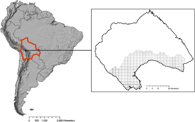
Location of the study area (Southern Slope in light grey divided into 25-ha planning units), within the Tunari National Park (dashed outline in frame) in Bolivia (bold orange outline), South America. Map created using ESRI ArcGIS software version 10.1.

Full size image

MarZone framework

Marxan with Zones (referred hereafter as MarZone⁹), uses biodiversity features and economic costs to allocate land parcels called planning units to different land-use categories referred to as zones. MarZone is an extension of the decision support tool Marxan¹² with land use zoning options. MarZone is a complementarity-based algorithm which solves the minimum-set problem using simulated annealing techniques^8,9,22. Its main task is to find the best zoning plan to meet a set of user-defined biodiversity targets, while minimizing the total cost of the solution.

We divided the study area into 4081 planning units of 25 ha-squares, which reflects a balance between the requirement for analytical time and the resolution of the environmental data available to obtain optimal solutions within reasonable computational time²³. Planning units were then allocated by the algorithm to different zones representing different possible uses. How much each unit contributes to reach the biodiversity targets depends on its current biodiversity value (the percentage suitability of the unit for each of the species and percentage of Polylepis cover, see below) and the zone to which it is allocated (through the zone contribution, see below). Each planning unit receives a cost for allocating the unit to one of the zones. Note that the analysis does not consider possibilities for habitat restoration; therefore, the current biodiversity value of a planning unit cannot be increased.

Biodiversity features and targets

We used two categories of biodiversity features in the analysis: one habitat feature (actual Polylepis woodland cover), and the habitat suitability for 35 bird species (Table 1) occurring in Polylepis woodlands in our study area (i.e. species for which shrubland and forest habitats are considered either major or suitable to the species according to BirdLife International²⁴ and/or recorded regularly within the surveyed Polylepis woodlands, see extended methods S1). Of these species, three are considered Polylepis-dependent species as they rely on the tree species to feed and five species are considered Polylepis-associated species as they occur in Polylepis habitats throughout their range²⁵ (Table 1). We calculated the Polylepis cover as the percentage of current Polylepis forest cover per planning unit, estimated from a Landsat 8 image (30*30 m resolution, see extended methods S2 for details). Habitat suitability models for all 35 bird species were generated from occurrence data collected in the field (see extended methods S1 for details) using the Maxent methodology (version 3.1; http://www.cs.princeton.edu/~schapire/maxent/²⁶. To prevent the selection of unsuitable habitat by MarZone, we thresholded each species’ continuous habitat suitability estimates using the True Skill Statistics (TSS²⁷). For each species, values located below the threshold calculated (Supplementary Table S1), were converted into 0 values while values above the threshold remained unchanged to reflect ‘true’ suitability²⁸. The habitat suitability value per planning unit was then calculated from the thresholded maps, as the mean suitability per planning unit for each of the bird species.

We calculated the target of each biodiversity feature based on its conservation priority²⁹. To test how targets affected land-use zoning, we ran three different scenarios with different target ranges for biodiversity features depending on their conservation priority. We set arbitrary minimum and maximum targets as 20% and either 50%, 75% or 90% of the total amount of each biodiversity feature with lowest and highest conservation priority, respectively. For features with intermediate conservation priority scores, we applied a linear scale to the total species scores from a minimum of 20% up to either 50%, 75% or 90% (Table 1). Conservation priority was defined as follows: for each bird species, a score of 1 was given for country endemism, IBA trigger species, EBA trigger species and small range size (<75000 km², BirdLife International²⁴). Additionally, a score of 1 and 2 were given, respectively, to species classified as Near-Threatened or Endangered by IUCN³⁰. We systematically assigned the maximum target for Polylepis cover (i.e. 50%, 75% or 90% of current total cover distribution, depending on the scenario).

We built six scenarios with the three target ranges, applied to scenarios with either four or five zones (Table 1), which we named ‘4z50’, ‘4z75’, ‘4z90’, ‘5z50’, ‘5z75’ and ‘5z90’. For each scenario, we used the best solution (zoning plan) found by MarZone from 100 iterations and calculated its achieved biodiversity value. The achieved biodiversity value of each zoning plan is calculated as the average of all habitat suitability and Polylepis forest cover percentages conserved in the zoning plan across planning units. This achieved biodiversity value was later plotted against the estimates of ecosystem service delivery to identify synergies and trade-offs (see below).

Land use allocation rules

We identified five different land use zones to which planning units could be allocated by MarZone. Three of the land-use zones were based on the most common extractive land use types carried out in the study area: agriculture, grazing and forestry zones. The agriculture zone includes intensive, extensive or subsistence agricultural practices primarily aimed to grow potatoes or cereals (see Extended Methods S3 for details). In practice, the type of agricultural practices carried out in the zone is constrained by altitude, slope and water availability¹⁹. In the grazing zone, animal husbandry with sheep or cows is practiced, while forestry refers to the establishment of dense exotic tree plantations. We included a fourth zone, the conservation zone, which represents a strictly protected strategy, with no further human exploitation allowed. Since it has been suggested in previous local studies that agroforestry practices (fields planted with native trees such as Polylepis) would be beneficial both for biodiversity and ecosystem service delivery^17,31,32, we ran an additional set of scenarios in which we included a fifth agroforestry zone. Finally, 6% of the study area, mainly covered by rocks and unsuitable for anthropogenic use, were locked into a static bare zone and retain any biodiversity value they may have.

To ensure land use allocation remains realistic, we established land use allocation rules for each planning unit based on the current land cover (derived from the classified Landsat image mentioned above, Supplementary Fig. S4) and the best potential land use (Supplementary Fig. S5). The best potential land use was extracted from a map previously published¹⁹ based on local expert knowledge and data on topography, vegetation cover and soil characteristics. We determined the best potential land use for each planning unit as the most dominant best potential land use within that unit. As the best potential land use is constrained by the properties or capacity of the land (i.e. only high-quality land can be used for agriculture while steep areas or poor soils can only be used for grazing and forestry purposes), we established four allocation rules: (1) all planning units can be allocated to the conservation zone; (2) planning units with agriculture as best potential land use can be allocated to any zone; (3) planning units can be allocated to forestry and grazing if their best potential use is either forestry or grazing; (4) any planning unit can be allocated to agriculture or grazing if it is currently covered by puna grassland/agricultural fields and to forestry if it currently contains exotic plantations.

Contribution of each land use to conservation

We used the zone contribution feature of MarZone to specify how the value of biodiversity features of each unit contributes to the targets when allocated to a specific zone. As planning units allocated to the conservation zone or to the bare zone are assumed to be unaffected by land use, their biodiversity values are also unaffected, and we assigned a 100% contribution value to both zones for all features. Both forestry and grazing zones were assigned a 0% contribution for all features, as forestry (which is exclusively carried out with exotic tree species) and grazing practices strongly impact and may ultimately displace native vegetation and its avifauna^31,33,34,35. For agriculture and agroforestry, zone contributions were differentiated among bird species based on our own detailed observations on bird habitat use in the Polylepis-agriculture mosaic habitats characteristic of the study area (Fastré et al., in prep) in combination with literature data^36,37,38 and BirdLife habitat classifications²⁴. Combining data from these different sources, we classified the species by their habitat affinity into three categories: species observed (1) exclusively in forested habitats (native forests), (2) in both forested and agricultural habitats and (3) mainly in agricultural habitats. We arbitrarily assigned contribution values of 0, 50 and 100% to the agricultural zone for bird species in each respective category. We further subdivided species observed in both forests and agricultural habitats into species with (2a) higher affinity for forest, (2b) equal affinity for both habitats and (2c) higher affinity for agriculture. We assigned contribution values of 100, 80, 60, 40 and 20% to the agroforestry zone for bird species belonging to categories (1), (2a), (2b), (2c) and (3), respectively (Table 1).

Costs of planning units

We estimated the opportunity cost of planning units as the loss of potential benefit to landowners of practicing a specific land use instead of the best potential land use. For this we converted the best possible land use map¹⁹ to a one-hectare resolution raster, using the most common land use as new land use per one-hectare pixel. From the same study, we derived values (in USD per hectare) for the maximum potential benefit of the land uses corresponding to the different zones (Table 2). We arbitrarily estimated that the potential monetary benefit of agroforestry, for which we did not have any value, would be 80% of the corresponding agricultural land use. We calculated the opportunity cost per hectare as the difference between the maximum potential benefit of the best possible land use, and the land use potentially allocated by MarZone (Table 2). We summed costs per hectare within each 25-hectare planning unit to obtain the values used in the analysis.

Ecosystem services modeling

We used the web-based tool AguAAndes (http://www.policysupport.org/aguaandes), a process-based hydrological model which incorporates detailed spatial datasets at one square kilometer and one hectare resolution for the Andes and scenarios for biophysical and socioeconomic processes and climate, land use and economic change to support hydrological analysis and decision-making in these data-poor areas^{39,40,41,42,43}. We modeled four water-related ecosystem services that have high relevance for the study region¹⁹: (1) erosion leading to agricultural capacity loss, estimated by net soil thickness loss (mm/year); (2) flood risk in areas beneath the slope caused by water runoff, estimated by total surface water runoff (m³/year); (3) water stress, estimated as the percentage of non-agricultural unmet water demand which can reflect long-term underground water reserves depletion; and (4) water pollution estimated as the percentage of water potentially contaminated by human activity.

We developed a baseline model for each service (Supplementary Figs. S6–S9), representing the current situation, which was calculated using globally available and remotely sensed data. The hydrological baseline is simulated as a mean over the period 1950 and 2000³⁹. Baseline total values of erosion (mm/yr), runoff (m³/yr), water stress (summed %) and water pollution (summed %) were calculated and compared with the values calculated for the land use plans generated with MarZone (see below). This modeled baseline situation represents ecosystem services in a study area that would be entirely conserved in its current state. We then used simulations to evaluate the effect on each ecosystem service of converting the entire study area to each of the zone used in the zoning plan. To assess the effects of (agro)forestry and grazing, we simulated ecosystem services under afforestation and conversion to grasslands, respectively. To assess the effects of conversion to agriculture we simulated deforestation to model erosion and runoff, because cultivated fields remain devoid of any vegetation cover most of the year. However, since crop cover and agricultural practices such as irrigation may have strong effects on water stress and pollution, we modeled these two services under simulated conversion to croplands.

To obtain the values of ecosystem services for the different zoning plans obtained previously, we overlaid the planning units allocated to each zone in each of the MarZone solution with the corresponding ecosystem service simulation (afforestation for forestry and agroforestry, deforestation or crop conversion for agriculture, grassland conversion for grazing and baseline situation for the conservation and bare zones). We summed ecosystem service values of the different zones to estimate the total values of erosion (mm/yr), runoff (m³/yr), water stress (summed %) and water pollution (summed %) for each zoning plan generated with MarZone. We also calculated the change in delivery of these ecosystem services compared to the current situation as the difference between the baseline situation and the new values per zone and for the entire study area. Finally, to identify potential trade-offs, the summed ecosystem service values of each zoning plan were plotted against the average achieved biodiversity value.

Source: Ecology - nature.com