Being able to compare travel modes to each other (realistically) at different hours of the day requires following a so-called door-to-door approach (Fig. 1). This means that travel time and distance are calculated comparably between travel modes by considering every step of a journey when calculating a route between origins and destinations. These steps include walking legs and transfers from one vehicle to another and the time it takes to search for a parking space or lock/unlock one’s bike. Considering these steps makes the travel times between transport modes more comparable with each other, and realistic measures of accessibility can be provided.
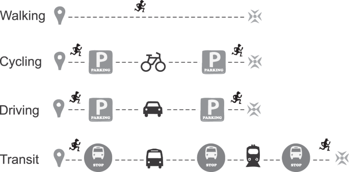
In door-to-door approach, every step of a journey in different travel modes is considered.
A variety of input datasets (Table 1) and methods were used to capture and model accessibility for different travel modes in a dynamic manner at different hours of the day. Figure 2 represents a generic workflow for producing the data. Specific preprocessing steps were applied for private car and cycling analyses to improve incorporation of the spatio-temporal dynamics of travel. After the initial pre-processing step, dedicated graphs were built for different travel modes that are required to calculate the shortest path routes between locations in the study area. Finally, the results were parsed and harmonized into a systematically formatted matrix, and the data quality was assessed against other data sources. The next sections provide further details about the analytical approaches used for each travel mode. Details on how to reproduce the data can be found at helsinkimatrix.github.io including processing codes and source data.
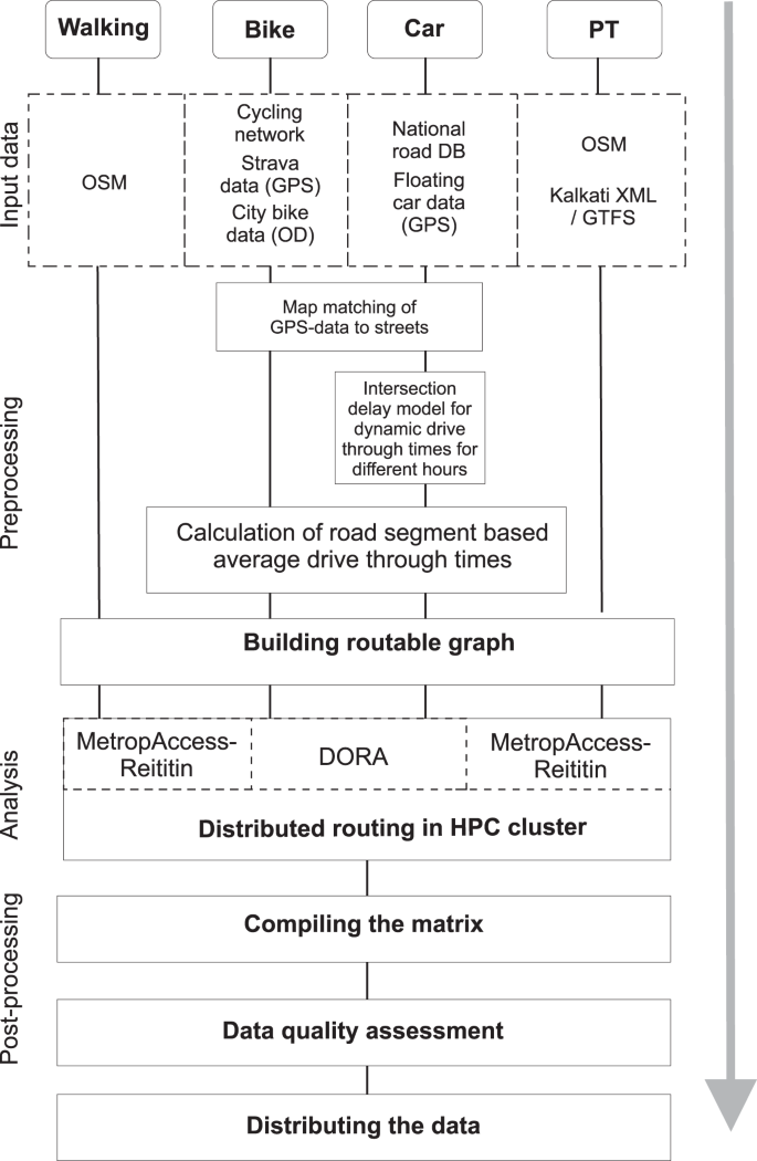
Generic workflow of the analytical steps that were taken to produce the travel time and distance data for Helsinki Region.
Travel time calculations
Travel time and distance calculations were done separately for each travel mode: public transport, private car, cycling and walking. Furthermore, the calculations were conducted separately for the morning rush hour (08:00–09:00) and midday (12:00–13:00) times, to be able to understand the dynamism of the transport system due to changes in timetables and congestion levels on the roads. The centroids of the statistical grid cells (Fig. 3) were used as origin and destination points for the calculations, covering the cities of Helsinki, Espoo, Vantaa and Kauniainen. The statistical grid (helsinkimatrix.github.io/grid) was originally created by Statistics Finland and the Finnish Environmental Institute (FEI), and it has the ETRS89/ETRS-TM35FIN projection. Hence, the data can be directly used with statistical data obtained from these institutions.
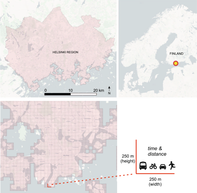
Dataset covers the Helsinki Region in Finland where the area has been divided into 250-metre statistical grid cells. Each grid cell contains information about the travel times and distances to every other cell in the area by public transport, car, bicycle and walking. Background map courtesy of OpenStreetMap contributors and Carto.
Public transport
A dedicated tool called MetropAccess-Reititin (helsinkimatrix.github.io/reititin) was developed for public transport routings. As input data, MetropAccess-Reititin uses Kalkati.net XML data14 that is a specific data format used by Helsinki Region Transport for publishing public transport schedules, stops, routes etc. OpenStreetMap data were used for walking paths including areal features such as squares and plazas, and the data were obtained from Geofabrik15 in Protobuf format. MetropAccess-Reititin is written in JavaScript and it uses a modified Dijkstra’s algorithm that considers transit timetable information when finding the optimal public transport route between given origin and destination locations (see16 for details). MetropAccess-Reititin is openly available from helsinkimatrix.github.io/reititin.
The tool considers the entire travel chains (following the door-to-door approach) from the origin to the destination (see also Fig. 1):
possible waiting at home before leaving
walking from home to the transit stop
waiting at the transit stop
travel time to next transit stop
transport mode change
travel time to next transit stop
walking to the destination
When routing, the tool first searches for the closest street edge from the origin (based on Euclidian distance). Following the network, it then finds 3–5 closest public transport stops, and considers all available transit options from those stops to find the fastest route between the given origin and destination points (for the given departure time). If the origin and destination are close to each other, the tool uses walking as the fastest route (whenever walking is faster than taking any of the public transport options). Walking speed was determined as 70 metres per minute. The tool stores detailed information about all steps of the journey that makes it possible to derive information about the exact distances for each travel mode. This makes it possible for example to calculate the CO2 emissions produced when using transit (see e.g.17,18).
For the travel time calculations, we obtained pareto optimal routes (due to varying departure times), by using ten departure times within the calculation hour using the so called Golomb ruler (departure minutes: 0, 1, 6, 10, 23, 26, 34, 41, 53, 55). The Golomb ruler makes it possible to gain maximal representation of departure times within one hour. The fastest route from these calculations is selected for the final travel time matrix. The travel times were calculated separately for the morning rush hour and midday on a typical work day using the effective schedules for those hours and days (see Table 2). Detailed documentation and instructions how to reproduce the public transport travel times/distances can be found at helsinkimatrix.github.io/pt_analyses.
Private car
For private car analyses, we first developed a dedicated intersection delay model (see19 for details) to generalise and associate the effect of congestion for the whole street network. In the model, we used GPS data from floating car measurements to understand how much congestion reduces driving speed at different parts of the study area (at different times). The deceleration effect of congestion is associated into the network by applying intersection penalties for different road classes and intersections. Hence, e.g. ramps at motorways have different intersection penalties compared to intersections affected by traffic lights on local main streets. By running the network through the intersection delay model, each road segment is given a different drive through times at different times of the day (rush hour, midday, whole day average, and speed limit based “freeflow” drive through times). The floating car measurements were collected by Helsinki Region Transport and the City of Helsinki. Preprocessed car network can be downloaded from helsinkimatrix.github.io/car_network.
When running the analyses with the modified street network, we followed the door-to-door approach, which includes:
walking time from the real origin to the nearest network location (based on Euclidean distance)
average walking time from the origin to the parking lot
travel time from parking lot to destination
average time for searching a parking lot
walking time from parking lot to nearest network location of the destination
walking time from network location to the real destination (based on Euclidean distance) See also Fig. 1.
For considering the time that it takes to walk to the car from home, we used values based on previous research conducted in Finnish city regions20,21. The distance was set as 180 metres (~2.5 minutes) in the city centre areas of Helsinki, and 130 metres in other areas (~2 minutes). The time that it takes to find a parking lot, was also based on previous literature21, and it was specified as 0.42 minutes across the study area. Calculations were done separately for two times of the day following rush hour (08:00–09:00) and midday (12:00–13:00) traffic conditions.
The calculations for 2018 were done with a dedicated open source tool called Door-to-door Routing Analyst (DORA) that was developed on top of PostGIS database v.2.3.3 (PostGIS community, 2019). DORA (helsinkimatrix.github.io/dora) is an open source multimodal routing tool that uses door-to-door approach when retrieving travel times between multiple origins and destinations. It can be used to route car, cycling and walking routes and is able to read any road network setup in a database with the pgRouting v2.3.2 (pgRouting community, 2019) extension. Detailed documentation for reproducing the data can be found at helsinkimatrix.github.io/car_analyses. Car routing for 2013 and 2015 was conducted with the ArcGIS v.10.1 (Environment Systems Research Institute, 2012) Network Analyst tool using a dedicated toolbox developed for the purpose. The ArcGIS toolbox (requires ArcGIS -software) is openly available at helsinkimatrix.github.io/md-tool. We ensured that the DORA and ArcGIS routing tools produced similar results, making the datasets between the years comparable; see helsinkimatrix.github.io/dora_validation for further details.
Cycling
For cycling analyses, we built a customized routing network called MetropAccess-CyclingNetwork by utilising GPS data from the Strava sport tracker application from 2016. The Strava dataset is based on data from 5223 unique users. We first linked the GPS points to the closest streets by using customised map matching techniques22,23. We then identified the roads that are most commonly used by cyclists and calculated user-based cycling speeds for different road segments. Finally, we aggregated this information into an average travel speed per segment. See22,23 for details on how the Strava data was processed.
Since the cycling speed is heavily influenced by personal characteristics of the cyclist (e.g. gender, fitness, age, etc.), the cycling speed we identified was not used directly. Instead, we associated each road segment with information about how much faster or slower the cyclists typically ride at a given road segment compared to the total average travel speed across the network according the Strava data. For instance, segment A is ridden 10 percent faster than on average, and along segment B the speeds are typically 5 percent slower than the baseline average speed.
Once the speed profiles were linked to road segments, we calculated ride through times by using the average cycling speed (19 km/h) of Strava sport tracker users as the reference value for “fast cyclist”. We also calculated separate ride through times for “slow cyclist”, in which we used the average cycling speed of a city bike system users (12 km/h). The average travel speed for city cyclists is based on data from a highly popular bicycle sharing system (BSS) in Helsinki. The data contains information about the origin and destination bike station, as well as distance travelled and the time it took. This information was used to calculate the typical travel speed of city cyclists. We also included extra time (1 minute) for unlocking and locking the bike, in order to follow the door-to-door principle. The unlocking/locking time is a naïve measure, as it is the same for every location. However, because of this, it is easy to modify the time if needed, or if more accurate information is available.
Due to privacy reasons and our licensing agreement with Strava, we cannot publicly share the raw Strava data. However, the preprocessed cycling network that contains segment wise travel speeds based on Strava data can be downloaded from helsinkimatrix.github.io/bike_network. The Python scripts that were used to produce the cycling network can be found at helsinkimatrix.github.io/bike_preprocess. Documentation for reproducing the cycling travel times and distances with DORA routing tool is available at helsinkimatrix.github.io/bike_analyses.
Walking
The walking routes were calculated using the MetropAccess-Reititin by disabling all motorised transport modes in the calculation. Thus, all routes are based on the OpenStreetMap (OSM) network obtained from15 at the time of the analysis. OSM is a good data source for estimating pedestrian travel times especially in urban areas24, as the data contain paths that are not available in the national road network (which is specifically targeted at car drivers). We used a static walking speed of 70 metres per minute (4.2 kilometres per hour) that is also used by public transport journey planner in Helsinki Region (reittiopas.hsl.fi). The same walking speed was applied also for the walking legs in the public transport calculations. Further details on how to reproduce the data for walking can be found at helsinkimatrix.github.io/walk_analyses.
Source: Ecology - nature.com
