In this section, we use the network models proposed in the Methods section to understand aspects regarding the taxonomic preferences and the collecting behaviour of collectors who have contributed to the University of Brasília (UB) Herbarium with specimens records.
Data
In this case study, we have used the entire digitized collection of records from the UB Herbarium23, which is publicly available for download through the Global Biodiversity Information Facility (GBIF) data portal24. We have used the Python v.3.6 language loaded with packages Pandas, Numpy, and Matplotlib for exploring the occurrence dataset; and the Caryocar package (designed and implemented by us, in the context of this work) for programatically constructing the SCN and CWN models from occurrence data. At the time of this study, the entire occurrences dataset from the UB herbarium had a total of 185,311 records and 235 fields, covering records from 1800 to 2017, although approximatelly half of the records are from the last 30 years (1988–2017). For our application, however, only a small subset of those fields were considered to be relevant and were thus included in our analysis: recordedBy, eventDate, stateProvince, countryCode, decimalLatitude, decimalLongitude, issue, scientificName, and taxonRank. Most of these fields (except for issue, which describes data quality issues found in the dataset) follow Darwin Core terms standards25.
Before we could use the UB Herbarium dataset for actually building the network models, we submitted the tabular dataset to some data filtering and transformation routines. The data preparation process consisted of (i) selecting occurrence records from which relevant social ties could be derived for both network models; (ii) extracting atomized collector names from the recordedBy field, which originally contains a string of names; (iii) normalizing the extracted collector names to obtain their id’s; (iv) resolving inconsistencies on collector names and mapping name variants to entities; and (v) filtering out inadequate collector names. All this data pre-processing, data cleaning routines, and data transformation is done by the code available in the Caryocar package. All the presented analyses used the dataset from Munhoz et al.23 and our package (examples on how to do it are provided with the package as well). The result is the SCN and CWN models we further discuss in the remainder of this section. In the presented figures, for a richer visualisation experience26, we also add links to browsable interfaces that reveal the scale and complexity of the represented networks.
The UB Species-Collector Network
The UB SCN model has a total of 6,768 collectors and 15,344 species nodes, with a total of 142,647 undirected edges connecting nodes from opposite sets.
Connected components
The UB SCN is composed of a total 351 connected components, the largest of which (the giant component, or c1) contains the majority of nodes in the network (93.6% of the collectors and 95.0% of the species). From a collector’s perspective, the requirement for it to belong to the giant component is that it must have collected at least one species in common with another collector who is already included in the giant component. The same reasoning applies to species nodes, by observing the inverse relationship. Apart from the giant component, most other connected components contain as few as two or three nodes, representing collectors who have never recorded a species in common with any collector from c1; and conversely, species that have never been collected by any of those collectors that belong to c1. One of those 350 remaining connected components, however, is considerably larger than the others, with a total of 3 collectors and 141 species. We refer to it as the second largest component (c2). Further, c1 is mostly composed of species from phylum Tracheophyta (88% of all records), followed by phylum Bryophyta (mosses), comprising 8% of the records. Component c2, on the other hand, is represented by algae (phyla Charophyta, Chlorophyta, comprising 91.6% of all records), bacteria (phylum Cyanobacteria (4.3%)), and other microscopic eukariotic organisms (phyla Euglenozoa, Myzozoa (4.1%)), which are taxonomically distinct from the vast majority of species in the herbarium. The remaining components (c3, c4, . . . , c351) include a total of 431 distinct collectors and 446 distinct species.
Communities of common interests
Communities in SCNs are formed by groups of collectors who are more interested towards particular subsets of species than are other collectors, external to the group. As the number of edges linking members of a community with other members tends to be larger than those connecting members to non-members, communities can be visually detected as distinguished clusters of nodes in the network when using force-directed algorithms27 for graph layout, thus no community detection algoritm was needed.
As the size of the UB SCN is relatively large for it to be informative in a static figure, we summarized the network in two steps. First we aggregated the SCN onto the family rank, as it would be impractical to draw relevant conclusions from the network if every single species were plotted in the figure. By performing the taxonomic aggregation, we reduced the number of Ssp nodes (taxa) from 15,344 to 474, although the number of edges (from 142,647 to 43,803) did not decrease in the same proportion. This incurred in a 10 × increase in network density, from 1.37 × 10⁻³ to 1.36 × 10⁻². In the second step of the summarization routine, we removed collector-family ties that occurred less than 20 times throughout the entire dataset. As this edge filtering routine resulted in many isolated collectors, most of which novice collectors with low absolute recording counts, we also omitted them as to improve the figure readability. Three communities are visually distinguishable from the central region of the network, which we refer to as the network core (Fig. 1). Although the network core could be considered a community per se, we prefer to think of it as a region that best reflects the overall interests of the majority of the collectors contributing to the herbarium. Nevertheless, collectors from the network core still vary considerably regarding their recording interests, as it can be verified by inspecting the sets of taxa they’re linked to and the strength of their connections. Those who have sampled organisms from many distinct families (and are thus considered to display a more generalist collecting behaviour) are placed more centrally in the network core by the graph layout algorithm, whereas those who are more specialists are consequently pushed towards the borders of the network core, as near as possible to their most recorded taxa.
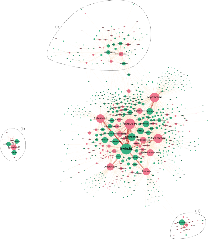
General aspect of the UB SCN, taxonomically aggregated at the family rank. Species and collector nodes are colored in pink and green, respectively. Node size is proportional to how often a collector or specimen appears on records, whilst the width of edges reflect their weight. Polygons (i), (ii), and (iii) are placed around communities that are visually most distinguishable. This figure has been originally presented in the first author’s MSc thesis28. For a better visualization experience refer to the interactive version of the graph (https://lncc-netsci.github.io/pedrocs/networks/ub_scn).
Represented as the biggest hub in the network, Howard S. Irwin (irwin,hs) is the collector with most records in the network, having intensively collected organisms from many distinct families, especially from the most central ones (illustrated in Fig. 1 as the largest pink nodes in the network core). The majority of his records are, in descending order, from families Fabaceae, Rubiaceae, Asteraceae, Poaceae, and Cyperaceae. He is also the collector holding the highest number of records for those families in the UB Herbarium. An interesting fact is that although Myrtaceae is the second most recorded family in the dataset (with a total of 10,951 records), it was relatively overlooked by ‘irwin,hs’, having himself contributed with only 399 Myrtaceae records. The main Myrtaceae collector in the herbarium is Jair E. Q. Faria (faria,jeq), who apparently has a preference towards this family (it comprises 31.0% of his entire set of records). Carolyn E. B. Proença (proenca,ceb) is another key Myrtaceae collector, although she also seems interested, to the same extent, in families Fabaceae and Asteraceae. Moreover, Fig. 1 also makes it easy to detect collectors who exclusively (or almost exclusively) collect each family, as it is the case of Vanessa G. Staggmeier (staggmeier,vg) for Myrtaceae and Regina C. Oliveira (oliveira,rc) for Poaceae, for instance.
Community (i) in Fig. 1 represents a large part of the collectors from Cryptogams Lab, together with the taxa they are typically most interested in. This lab is part of the University of Brasília Department of Botany, having Paulo Eduardo A. S. Câmara (camara,peas), Micheline C. Silva (carvalhosilva,m), and Maria das Graças M. de Souza (souza,mgm) as the principal investigators. The first two researchers, included in community (i), are mostly interested in bryophytes (mosses and liverworts), mainly those from families Sematophyllaceae, Hypnaceae, and Dicranaceae. Micheline C. Silva also shows interest towards Piperaceae, a family of flowering plants that is also fairly recorded by some collectors from the network core. Therefore, Piperaceae is an important node connecting community (i) to the network core, as it intermediates many paths between collectors from both network regions. Although she is one of the principal investigators of the Cryptogams Lab, ‘souza,mgm’ was placed in community (iii), instead of (i), due to her taxonomic interest towards algae, a taxonomic group that is overlooked by the vast majority of collectors in the UB Herbarium, including bryophytes collectors. She is mostly interested in families Eunotiaceae, Naviculaceae, and Pinnulariaceae, which compose a group of algae known as diatoms.
The UB Collector coWorking Network
As the UB CWN was built based on the same set of records as the SCN model explored in the previous section, the number of nodes is 6,768, equivalent to the number of collectors nodes in the SCN model. A total of 10,391 edges represent collaborative ties between collectors. The average degree and density for the overall network are, respectively, 3.07 and 4.5 × 10⁻⁴.
Connected components
The UB CWN is composed of a a total 2,991 connected components, the largest of which (i.e., the giant component c1) contains 46% of all nodes in the network. Such a relatively low percentage of nodes in the giant component contrasts to most empirical scientific paper-publishing collaboration networks studied by Newman29, with giant components containing as much as 80% to 90% of all nodes. Moreover, only 318 of the connected components in the UB CWN (c1, c2, …, c318) are composed of collectors with at least one collaborative tie. The remaining 2,673 components (c319, c320, …, c2991) are all disconnected nodes (i.e. nodes with degree k = 0), which we refer to as individualist collectors. Individualist collectors are those who have never recorded specimens collaboratively—or at least they have not included the names of their collaborators in the records as authors—, and thus are considered to have no structural role in the collaboration network of collectors. They comprise 39.5% of all nodes in the network, and the fact that they lack connections impacts on the overall network density, making it relatively low. In fact, if we instead compute network density by only considering nodes from the giant component c1, we observe an increase in density from 4.5 × 10⁻⁴ to 1.95 × 10⁻³.
One important example of an individualist collector in the herbarium is ‘leite,alta’, with a total of 2,757 records, none of which recorded as made collaboratively. This comprises 18.14% of all records by individualist collectors. All other 2,672 individualist collectors have fewer than 400 records each.
How collaborative are collectors
By inspecting the team sizes of all records in the dataset, we find that the average team size for records in the UB dataset is 1.73, as a consequence of the fact that a large part of all records are non-collaborative, i.e. recorded by a single collector. The number of records as a function of team size seems to decay logarithmically. Collectors from the UB Herbarium vary substantially regarding their collaborativeness on fieldwork. Whereas few ones have collaborated with a large number of collectors throughout their careers (much more than the average 3.07), many of them hold very few collaborative ties. In fact, almost 40% of them are individualist collectors, having never co-authored a single record.
The vertex betweenness centrality metric is also frequently used in social network analytics for ranking nodes that act as “bridges”, intermediating a considerable fraction of shortest paths between pairs of nodes in the network. We compute betweenness centrality of a node v by making ({c}_{B}(v)={sum }_{s,t}frac{sigma (s,t| v)}{sigma (s,t)}), where V is the node set; σ(s, t) is the number of shortest paths between nodes s, t ∈ V (both s and v different from v); and σ(s, t ∈ v) is the number of shortest paths between s and v that are pass through v30. The 4 collectors with the highest betweenness centrality scores in the UB CWN are ‘proenca,ceb’ (0.38), ‘faria,jeq’ (0.18), ‘mendes,vc’ (0.14), and ‘ratter,ja’ (0.13). By inspecting Fig. 2, we verify that in fact all those collectors are in strategic positions. Carolyn E. Proença (proenca,ceb) is located at the center of the network, while ‘mendes,vc’ and ‘faria,jeq’ also interconnect nodes from many distinct communities. James A. Ratter (ratter,ja) is a very important node bridging a very relevant group (the green one, around ‘irwin,hs’) to the remainder of the network. Through the diversity of connections they had with other collectors, this top collectors from the betweenness perspective act as “bridges” connecting different communities of collectors.
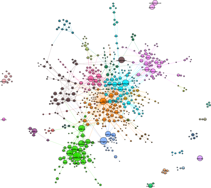
General aspect of the UB CWN. A total of 30 distinct coworking groups have been identified, and are differentiated by color. Node size is proportional to how often a collector appears on records, whilst the width of edges reflext their weight. This figure has been originally presented in the first author‘s MSc thesis28. For a better visualization experience refer to the interactive version of the graph (https://lncc-netsci.github.io/pedrocs/networks/ub_cwn).
Coworking groups
One important aspect that can be investigated from the topological structure of the UB CWN is the formation of communities of collectors who co-author specimen records, which we refer to as coworking groups. Nonetheless, visual inspection of the network structure does not allow us to fully identify the communities in this case. In order to detect such groups we applied the Louvain heuristic method for community detection31. The Louvain algorithm maximizes modularity scores in the network in successive steps, whereas the adopted modularity index is the one proposed by Newman32. The software we used for that is the python-louvain module for the NetworkX packagea.Footnote 1 The result is a partition of the network into modules (communities) within which nodes are more densely connected with each other than with external ones. Using this method, we detected a total of 30 distinct communities, 11 of which are detached from the giant component. For graph visualization, we first performed a filtering routine. We first filtered out weaker edges (those with hyperbolic weighting from Equation 3 lower than 10), which resulted in many islands, i.e. isolated components. We assigned scores to each island by summing up the weights of all nodes composing them. Islands with scores lower than 600 were omitted. The resulting graph has 545 nodes, 1,158 edges, and an average degree of 4.25 (Fig. 2). Among the communities, we identify the bryophytes research group, which includes ‘camara,peas’, ‘carvalhosilva,m’, and ‘soares,aer’. Collectors from this coworking group (colored in purple and located in the upper-right region of the giant component in Fig. 2) not only mostly collaborate with members from the same group in fieldwork, but they are also interested on recording the specific taxonomic group of bryophytes.
Source: Ecology - nature.com
