Protection of Permafrost Soils from Thawing by Increasing Herbivore Density

Snow depth observations, Northern Sweden

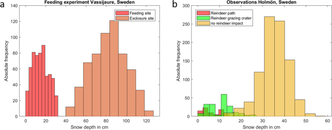
The effect of reindeer on snow depth has been measured in two study sites. The first is a large enclosure used for winter feeding of Norwegian reindeer (Gielas reindeer herding districts) in Northernmost Sweden, close to the Vassijaure railway station (68({}^{circ }2{5}^{{prime} }46.{2}^{{primeprime} })N,(1{8}^{circ }2{0}^{{prime} }47.{3}^{{primeprime} })E). Inside the enclosure, 700 reindeer were kept for 28 days in a 12 ha large enclosure during the winter 2017, corresponding to a density of 483 reindeer per km² during that period. Snow depth was measured at 16 April 2017, a couple of weeks after the reindeer had left the enclosure. Snow depth was measured with an avalanche probe every 10 cm along six transects inside the enclosure and six transects outside the enclosure (undisturbed by reindeer). The transects were paired in sites with similar topography to avoid confounding factors, and the difference inside and outside the enclosures should thus relate to the presence of reindeer only. The second study site is the Holmön archipelago (63({}^{circ }43.159{prime} )N,20°(55.078{prime} )E). The islands has occasionally been used as winter grazing area by Rans reindeer herding district. Between October 2015 and April 2016 about 700 reindeer were moved to the Holmön archipelago, which corresponds to a density of 15 reindeer per km². Here, snow depth was measured at 17 March 2016 every 10 cm along twelve 10 m long transects with the same methods as in the first study site. Each point along the transect was also characterized as no impact by reindeer, trampling, or feeding crater. The densities in both these study areas was much higher than the average densities of reindeer presently found in the Arctic of 0 to 10 reindeer per km²¹⁷. However, since reindeer are migratory and move in large herds, extreme densities corresponding to the enclosure is sometimes found for a few weeks also under natural settings, and the Holmön island is a natural use of winter resources and corresponds to densities often found in an area a year that is used for winter grazing.

Pleistocene park experiment, cherskii, russia

Pleistocene Park is the scientific experiment on reconstruction of highly productive steppe ecosystems in the Arctic¹⁹. The experiment is conducted in the Kolyma river lowland (68.51°N,161.50°E). It is a 2000 hectare area divided into subsections by game fences. Typical northern vegetation types- tussock grassland, willow shrubs and larch forest, originally represented the landscape. Starting 1996, different herbivores were introduced to the Park. Some species are native to the region, some used to inhabit the area in the Pleistocene. These are reindeer, Yakutian horses, moose, musk ox, European bison, yaks, cold adapted sheep. Density of herbivores is artificially kept above the feeding capacity of the pastures (by providing extra forage). This allows grasses and herbs to out-compete modern low productive vegetation and gradually increase productivity of the territory. To test the effect of winter grazing on snow cover and permafrost temperature, in 2011 soil temperature sensors in the year-round grassland pasture within the park and in the similar landscape but without grazing, 10 km outside of the park, have been installed. Temperature sensors were installed within the active layer on the depths of 10, 25, 50 and 90 cm. Nonstop temperature measurements were obtained from July 2011 to May 2013 for the non-grazed site and from July 2012 to July 2013 for the grazed site.

Land surface model

In this study we use a version of the land surface scheme JSBACH^22,36,37 that has recently been advanced by several processes which are particularly important in cold regions, including coupling of soil hydrology and vertical heat conduction via latent heat of fusion²⁰ and the effects of ice and water content on soil thermal properties²⁰, as well as a new dynamic snow model for soil insulation^21,25. The version used here in particular also includes a dynamic biogeochemical model of lichens and bryophytes²¹ which simulates both the extent of lichens and bryophytes and their impact on the vertical heat conduction^21,25. In total, five snow layers, one bryophyte/lichens layer, and seven soil layers are used in an implicit numerical scheme to solve the heat conduction equation with phase change^21,23. Depth of thermal and hydrological layers increase from 6 cm at the surface to 30 m for the bottom layer. In sum, these layers reach a depth of 53 m ensuring no temperature amplitude in the last layer. However, the hydrological layers are restricted to the depth until bedrock, which typically range between 0.5 and 4 m in northern permafrost regions at the landscape scale. In this study, this information is based on ref. ²⁶ as used in ref. ²⁷. Horizontal resolution of model results is due to the resolution of forcing data (see below). Climate and soil datasets with a grid cell size of 0.5 degree are applied. Four dominant land cover classes are considered in each of these grid cells³⁶. The coverage of these tiles has been estimated by combining several global land cover maps²⁰. JSBACH interpolates daily climate forcing data to half-hourly values which is the internal time step of the model. More details on the model version used can be found in refs. ^20,21,25. This model version has been intensively evaluated in terms of cold regions physical processes at site level and pan-Arctic scale^20,21,24,25. Additional evaluation plots can be found in the supplemental information.

The advanced snow module of JSBACH represents a dynamic snow density (ρ_snow. It is initialized with a minimum value of ρ_min = 50 kg m⁻³. The compaction effect is included as a function of time³⁸ with a compaction rate c = −0.002 and a maximum density (ρ_max = 300 kg m⁻³),

where Δt is the timestep length of model simulation in seconds. Snow density is calculated as a weighted mean of fresh snow with snow density (left({rho }_{min}right)) and the previous timestep’s value. Snow density controls snow heat capacity and conductivity²⁵ and snow depth. Both, snow thermal properties and snow depth impact the insulation characteristic of snow and hence soil temperature. A higher snow density (e.g. due to herbivore grazing in winter) leads to a higher heat conductivity hence stronger heat flux in winter (soil cooling), and a higher snow density also leads to a lower snow depth hence closer atmosphere-soil coupling in winter (soil cooling).

Climate forcing data

The JSBACH model driver estimates half-hourly climate forcing data using daily data of maximum and minimum air temperature, daily precipitation, short-wave and long-wave radiation, specific humidity and surface pressure. We are using global data at 0.5 degree spatial resolution. The historical data from 1901-1978 came from the WATCH forcing dataset³⁹ at the same resolution. For the period 1979-2010, ERA-Interim reanalysis data have been downloaded from ECMWF also at 0.5 degree grid cell size⁴⁰. This dataset has been bias-corrected against the WATCH forcing data. Climate data for future projections (2011–2100) have been obtained from the CMIP5 output of the Max-Planck-Institute Earth System Model³¹ following the RCP8.5. The original grid cell size of this dataset of 1.875 degree has been automatically improved to 0.5 degree by the bias-correction approach, which, in principle, projects the anomalies of the MPI-ESM time series onto a long term average of the reference dataset. For details about the bias-correction method please see refs. ^29,30. Historical and future atmospheric CO₂ concentration was prescribed following the CMIP5 protocol⁴¹.

Grid cells are divided into four tiles according to the four most dominant vascular plant functional types of this grid cell²⁰. This vascular vegetation coverage is assumed to stay constant over the time of simulation. Hydrological parameters have been assigned to each soil texture class⁴² according to the percentage of sand, silt and clay at 1 km spatial resolution as indicated by the Harmonized World Soil Database²⁸. Thermal parameters have been estimated²⁰ at a 1 km spatial resolution. Then, averages of 0.5° grid cells have been calculated. An updated map of soil depth down to the bedrock^26,27 has been applied.

Simulation protocol for CNTL and PlPark model experiments

Climate forcing during the spin-up time consisted of randomly selected years during 1901-1930 from the climate dataset described above. Pre-industrial atmospheric carbon dioxide concentration was assumed to be 284 ppmv. First, JSBACH has been run for 30 years without enabling the freezing scheme in order to bring soil water reservoirs in a first equilibrium with climate. Then, JSBACH was again running 170 more years with the same forcing data but with enabling the freezing scheme in order to equilibrate soil temperature, soil water and ice content as well as lichen and bryophyte cover according to pre-industrial conditions. Afterwards, the spin-up model for the carbon pools was run for 10 k-years using JSBACH output from the last 30 years of the pre-industrial spin-up run. JSBACH was then run from 1850 to 1900 using again the random spin-up climate from the period 1901–1930 but using transient atmospheric CO₂ concentration, followed by a fully transient run until 2100 using the climate data described above and dynamic atmospheric CO₂ content following the RCP8.5⁴¹.

JSBACH has been additionally run during 2021–2099 starting from the CNTL experiment state variable conditions in 2020 but with

• increased snow compaction rate (c = −0.003 h⁻¹),

• increased maximum snow density (ρ_max = 450 kg m⁻³), and

• a doubling of the moss turnover rate constant.

This simulation emulates an increase of big mammals, such as horses, reindeer, bison etc. in 2020 leading to increasing snow density, comparable to the Pleistocene Park experiment in Cherskii, Russian Far East. The experiment is therefore called PlPark. All other parameters and forcing data remain the same as in the CNTL simulation.

Definitions, data analyses and plotting

Mean annual ground temperature (MAGT) is calculated as an average of soil temperature in 4 to 10 m depth. In this depth the temperature is fluctuating only marginally. Permafrost temperature is defined as MAGT in permafrost areas. The model results are then spatially plotted and analysed over the northern permafrost area, which is defined by 1990–2009 or 2090–2099 permafrost temperature lower than zero degrees Celcius. All land outside this permafrost zone is marked in grey color. The area of all permafrost-defined grid cells is summed as a pan-Arctic estimate. Grid cells that are treated as permanent glaciers in the model are excluded from this analysis.

Parameter sensitivity study

In order to study the impact of snow and moss parameters on permafrost temperature and extent, the three parameters maximum snow density, snow compaction rate, and moss turnover rate have been varied simultaneously using a Latin hypercube sampling design resulting in 20 additional model runs. Ranges of possible parameter values are as follows: maximum snow density: 350–450 kg m⁻³, snow compaction rate: 0.002–0.003 h⁻¹, and moss turnover rate: 0.01–0.02 a⁻¹.

Source: Ecology - nature.com