The diffuse light around cities in nighttime satellite imagery of the Earth has often been interpreted as instrumental error. Here we have shown that this is not the case. Rather, this light is mostly due to sky brightness propagated from urban areas. This is quite an exciting result, as it means that, in principle, maps of sky brightness could be produced from satellite data.
The current state of the art in understanding the spatial variation of skyglow are maps produced by sky brightness models. While these are undeniably useful, the models have limitations, and in many cases experimental data would be preferred (e.g. for daily time series). Furthermore, obtaining sky brightness maps based on ground-based data is an extraordinary challenge. For example, Bara has demonstrated38 that interpolating a skyglow map accurately requires data with grid spacing of about 1 km. This would be difficult to accomplish with ground based observations, and is therefore the kind of problem that space-based mapping is well suited for.
Before maps of skyglow can be generated using space-based data, a better understanding of the relationship between skyglow observed from space and from the ground must be achieved. The variation between observed and DMSP predicted sky brightness reported here can be compared to that previously published by Kyba et al.19. In Kyba et al., the standard deviation of the residuals was ~0.5 magSQM/arcsec2, whereas here we observed 0.3 magSQM/arcsec2. A major difference between the two works is that Kyba et al. was based on observations obtained through a citizen science project. The improved accuracy in this paper can be attributed to several factors. First, the UCM sky brightness survey was performed by a single group of researchers using a single protocol and in similar weather conditions. In contrast, the citizen science data may include data from more turbid atmospheres, and the overly bright outliers in the citizen science data suggest that it was often taken too close to light sources. Also, the data from the UCM survey have been very carefully filtered to avoid false values. This issue is more difficult to address in a citizen science project.
When we analyze the residuals of all the observed sky brightness values and the predictions based on the fit between the satellite data and the UCM survey (see Fig. 5), we see the width of the main component is similar for all of them. The main difference between the different residuals is the shape of the tail to greater brightness. In the case of the DMSP data, the tail is not very pronounced, which we attribute to the large spatial size of its Point Spread Function (PSF). In the case of the other satellites, it is clear that the distribution is more asymmetric. (Note that for the DMSP satellite radiometer, the composite images do not show native resolution, but are rather based on averaging and super resolution methods23).
We further examined what happens at lower spatial resolution, by producing reduced resolution maps from the different satellite datasets, and then comparing these to the SQM observations. In all cases, we resampled the satellite maps to 15 arcseconds, 30″, and 60″. The changing relationship to the SQM observations is shown for DNB in Fig. 9, and for the two ISS photos in Figs. 10 and 11. As the resolution is reduced (i.e. pixel size is increased), the tail begins to grow and the size of the main peak decreases. We attribute this effect to the admixture of direct illuminated and diffuse illuminated signal within the same pixel. The sky brightness is more strongly related to diffuse light than to direct illumination, so as resolution is reduced information is lost. Histograms of the fit residuals at different resampled resolutions are shown for one of the ISS images in Fig. 12.
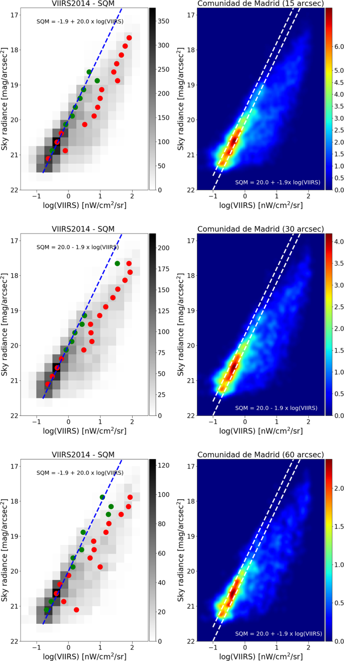
Relationship between sky brightness measured on the ground and satellite radiance observation for different sizes of pixel agglomeration for the VIIRS data. In the top plots, the VIIRS image data has been averaged over a pixel size of 15″ (arcseconds), in the middle plots 30″, and in the bottom plots 60″. In all cases, the relationship is strongest using the high resolution data. In the left plots, the green circle represents the dimmer Gaussian peak, and the red circles the brighter Gaussian peak. The right hand plots show the same result using a non-binned color coded density plot with a Gaussian filter. The two dashed lines have the same slope as the blue fit, and are shown for comparison purposes.
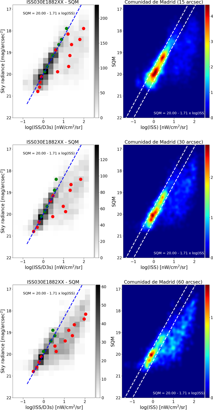
Relationship between sky brightness measured on the ground and satellite radiance observation for different sizes of pixel agglomeration, for ISS photo ISS030E1882. In the top plots, the ISS image data has been averaged over a pixel size of 15″ (arcseconds), in the middle plots 30″, and in the bottom plots 60″. In all cases, the relationship is strongest using the high resolution data. In the left plots, the green circle represents the dimmer Gaussian peak, and the red circles the brighter Gaussian peak. The right hand plots show the same result using a non-binned color coded density plot with a Gaussian filter. The two dashed lines have the same slope as the blue fit, and are shown for comparison purposes.
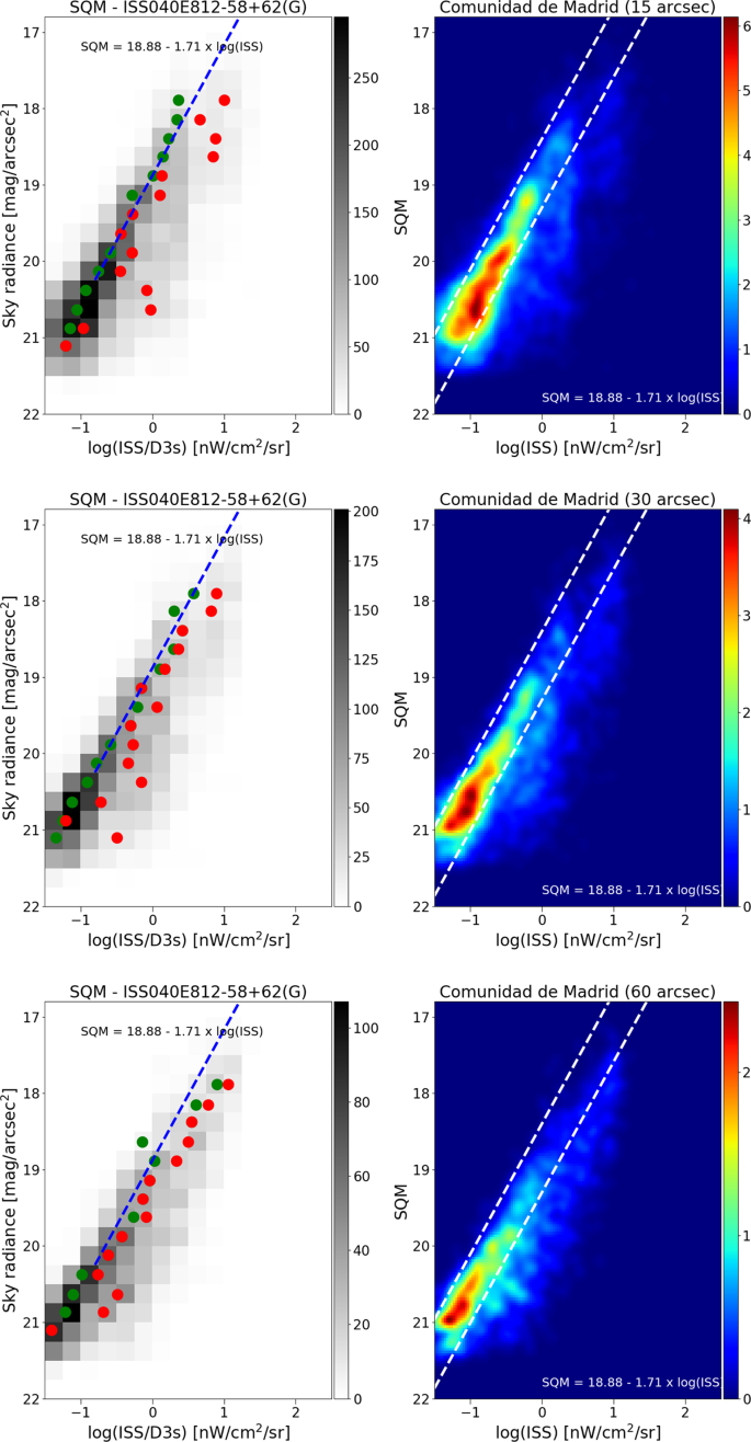
Relationship between sky brightness measured on the ground and satellite radiance observation for different sizes of pixel agglomeration, for ISS photo ISS040E0812. In the top plots, the ISS image data has been averaged over a pixel size of 15″ (arcseconds), in the middle plots 30″, and in the bottom plots 60″. In all cases, the relationship is strongest using the high resolution data. In the left plots, the green circle represents the dimmer Gaussian peak, and the red circles the brighter Gaussian peak. The right hand plots show the same result using a non-binned color coded density plot with a Gaussian filter. The two dashed lines have the same slope as the blue fit, and are shown for comparison purposes.
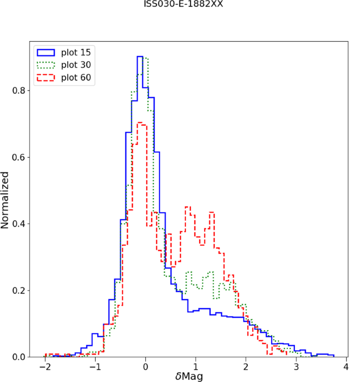
Impact of pixel agglomeration area on relationship between sky brightness and radiance detected from space. The histograms show the difference between the observed sky brightness and that predicted based on the ISS photograph. Larger values mean the sky is darker than would be expected. The relationship is best when the pixel size is smallest, or in other words, when the agglomerated pixel is small enough that it is unlikely to contain an admixture of both scattered skyglow and direct emissions.
We conclude that in the surroundings of Madrid and nearby municipalities, in most cases radiance values between 0.2–5 nW/cm2/sr are generally due to diffuse light. However, it is not possible to apply this as a land use classification, because direct light from small communities is frequently also in that range. Assuming that the Madrid data are representative of sky brightness in the rest of the world, this approach could be extrapolated more widely. As long as only broadband sensors are available, the correspondence between satellite radiance and skyglow will need to be adjusted locally, because the spectra of cities and types of light sources can differ.
In order to remotely sense skyglow using satellite imagery, other aspects of nighttime imagery such as natural sky glow (auroras and airglow), reflectance of the ground, thin cloud and fog, and transient lights, will also need to be studied in more depth. New sky brightness surveys are needed in areas sensitive to effects not considered by33, such as blocking effects of orography. For example, the circled area in Fig. 13 shows a significant difference between our model of skyglow based on VIIRS and ISS data (Fig. 7) and the sky brightness reported by the World Atlas. We believe this is most likely due to the mountains blocking the light of Madrid, resulting in a darker sky beyond them.
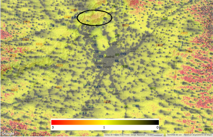
Ratio of our model of sky brightness based on VIIRS to the predictions of the World Atlas. In areas where VIIRS observes direct light the ratio is close to zero, as VIIRS is detecting direct rather than scattered light. In most areas near Madrid but outside of cities, the ratio is close to one. These are the areas where we believe VIIRS is observing skyglow, and values therefore match the World Atlas skyglow model. Some areas have higher ratios than one, for example the area North of Madrid which is circled. Our interpretation is that the World Atlas model is not correctly accounting for the blocking effect of mountains, as a large part of that area corresponds to the Sierra de Guadarrama National Park, and the Lozoya River basin, which is separated from Madrid by 1500 m high mountains. Computed with Google Earth Engine: https://pmisson.users.earthengine.app/view/tendsdiff (Source code available by request).
Recently, Simons et al.39 compared sky brightness measured via all-sky imagery to the World Atlas as well as to VIIRS radiance data. They found a higher correlation to the World Atlas than to the satellite data. This is to be expected based on the data in Fig. 13, as pixels containing a mix of direct and scattered light do not have a simple correlation with sky brightness (Differences between the World Atlas and our predictions based on DNB data can be viewed at https://pmisson.users.earthengine.app/view/tendsdiff). It would be interesting to see a similar study to Simons et al., but in places which have no direct light emissions. Observations from water bodies such as done by Jechow et al.40 are promising, but we caution that such studies should be done at least 1 km away from shore lights.
Temporal resolution
The focus of this paper is on the spatial distribution of skyglow, and not on temporal variation. However, light emissions are dynamic41,42, and produce changes in skyglow that can easily be detected26,43,44,45,46. This well known temporal variation acts as noise in this analysis, increasing the dispersion of the values. Sky brightness also changes over time due to changes in atmospheric properties (indeed, the relationship between diffuse light and the amount of aerosols47 provides additional evidence that the glow observed around cities is from real light).
Despite this, temporal variation can be effectively ignored here. Sánchez de Miguel26 presented an intensive analysis of the spatial, spectral and temporal variation of light pollution in Madrid and surrounding areas. The analysis found temporal variations with an amplitude of up to 0.3 magnitudes (~30%). Such variations are of second order compared with the spatial variation that can be up to 3 magnitudes (~factor 15).
The VIIRS, DMSP and ISS images also vary in terms of timing. The VIIRS data is based on the average statistics taken during several months, the DMSP data is based on the average statistics collected during a year, and the ISS images are nearly instantaneous samples at two moments in time. Ground based observations of skyglow can be either focused on temporal variation (stationary detectors) or spatial variation (with a moving detector). This study used moving detectors to cover a large area, and therefore the data were taken at different times in the night. Nevertheless, as discussed above, this effect is small compared to the spatial effect that is the key focus of this study.
Finally, we note that the DMSP data is taken during the early part of the night, whereas VIIRS data is taken well after midnight. If one were to restrict the comparison to skyglow data taken only during overpass times, it would greatly limit the spatial coverage that could be considered.
Other components of the diffuse light: albedo, natural airglow, sea fogs and real blooming
It is beyond the scope of this article to address all of the components of dim diffuse light that may be present in VIIRS images. However, we wish to make clear that not all of the diffuse light can be explained by the scattering of artificial light. Brighter diffuse areas appear in VIIRS images for a number of reasons, including natural airglow and aurora, areas with higher ground albedo or fog, and even an instrumental effect that appears similar to CCD blooming.
The sensitivity of the VIIRS DNB is so high that it can detect the reflectance of starry skies on the ground. We show the impact of albedo in Fig. 14. The region near the Wal al Namus volcano experiences among the most extremely rapid changes of albedo on the surface of the Earth. The figure shows the correlation between the median of the Albedo bands of MODIS and the VIIRS DNB for the four months closest to the second equinox (Aug to Nov), with data from 2012 to 2018. A clear correlation was observed (R2 = 0.93), although there is some structure that indicates that the spectral sensitivities of the VIIRS and MODIS do not match perfectly, so this result could be further improved. This effect was previously reported by Roman et al.48.
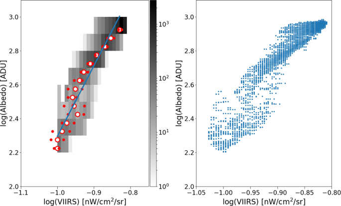
Correlation between the MODIS Albedo BSA Bands 1,2,3 and 4 and VIIRS median 2012–2018 in the proximity of the Wal al Namus volcano (Lybia).
The atmosphere naturally emits light that can be detected from the ground, primarily in a number of spectral lines49. These also contribute to sky brightness observed from space, but in a highly variable fashion because airglow is not constant from night to night. The area near the poles also has a permanent auroral ring around it.
Finally, higher than normal radiance is often observed in some areas of the ocean, and we believe this may be due to low level fog, thin clouds, or broken clouds that are smaller than the pixel size. These can be challenging to identify with the infrared channels of VIIRS, because they may have nearly the same temperature as the sea itself. The sea has a reflectance of less than 10%, while clouds have much higher albedos (e.g.50). There are often regions over the ocean with areas of diffuse light in the VIIRS monthly composites, and we believe this is due to fog or thin cloud that has not been identified in the cloud masking. This effect is most obvious near the equator between America and Africa, and in the northwest Pacific and northeast Atlantic (https://pmisson.users.earthengine.app/view/trends). This matches the areas of the Ocean that most often have cloud cover in the daytime VIIRS images (https://hannes.enjoys.it/carto/VIIRS_SNPP_CorrectedReflectance_TrueColor_median/).
Coming full circle, although the majority of diffuse light in nighttime imagery arises from sky brightening and not “blooming”, we have in fact occasionally observed an instrumental effect that appears similar to blooming. This is detectable in the high gain regime of VIIRS as tails to the distribution of brightness values that are a consequence of long exposure or blooming from the window of the instrument. This effect can be clearly seen in Fig. 15.
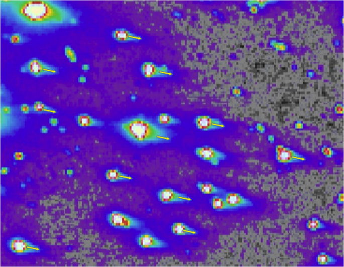
Blooming effect of dim sources near Villanueva de los Infantes, Spain (3.01°E, 38.65°N). This was based on finding the median value from 4 months in each calendar year, and then finding the mean of these values over 6 year.
Source: Ecology - nature.com
