Chemicals and materials
HPLC-MS grade water, acetonitrile, and methanol were obtained from Fisher Sci. Canada (Ontario, Canada). Formic acid, ammonium acetate, 37% hydrochloric acid, dimethylformamide, 150 kDalton polyacrylonitrile (PAN) were purchased from Sigma-Aldrich (St. Louise, Missouri, USA). The rare earth magnets were purchased from Lee Valley Tools (Waterloo ON, Canada). The 18-8 stainless steel springs, nuts, and bolts were purchased from Spaenaur (Kitchener, ON, Canada). Swagelok model 177-R3A-K1-B PTFE-coated springs were purchased from Swagelock Inc. (Sarnia, ON, Canada). The PTFE sampler bodies were constructed at the Science Machine Shop, University of Waterloo (Waterloo ON, Canada). The 5 µm and 30 µm, hydrophilic−lipophilic balanced (HLB) particles, which were used as functional particles in the coatings of the devices, were obtained by Waters (Wilmslow, U.K.)
Preparation of the coated bolt SPME devices
The first coated bolts were prepared using a spray coating methodology adapted from a procedure first reported by Musteata et al. and advanced by Mirnaghi et al.68,69. These bolts were used for sampling from the El Gordo vent. Briefly, this procedure entailed first dissolving 150 kDa polyacrylonitrile (PAN) in dimethylformamide (DMF) at a 10% PAN weight percentage, and then mixing 10 mL of the resulting solution with 1.0 g of 30 µm HLB particles and 3 mL of DMF so as to prepare a sprayable slurry. The surfaces of the stainless-steel bolts were etched by hanging the coatable surface of each bolt in an open beaker of concentrated HCl under sonication for 10 minutes. An Aldrich glass sprayer (Sigma-Aldrich, Oakville, ON, Canada) was used to apply approximately 10–12 coats of the slurry. Each coat was set in a modified GC oven at 150 °C. These coated bolts were then cleaned and conditioned in a 50:50 methanol: water solution.
For bolts prepared with a recessed extraction phase, which were used in the Urashima Field and Alba vent samplings, etching was performed for 1.5 hours, which resulted in a 30 µm indentation on the stainless-steel surface. Dip coating was then performed using a programmable actuator such that the bolts could be immersed in the aforementioned PAN/HLB/DMF slurry up to the edge of the etched surface. Furthermore, a smaller and more strongly sorbing 5 µm HLB particle was used for preparation of these coatings. The dip coating method entailed application of two coats of the slurry, with each coat being set in a modified GC oven at 150 °C. Thereafter, any excess coating was removed from the head of the bolt using a utility knife, whereupon the coating was cleaned and conditioned in a 50:50 methanol: water solution.
HLB/PAN TFME blades were prepared by dissolving PAN in DMF and preparing HLB/PAN slurries in the above concentrations for spray-coating on stainless steel blades, as described before by Mirnaghi et al.68.
Field sampling
We conducted three experiments to test the effectiveness of the self-sealing coated bolt sampler design for sampling at hydrothermal vent zones. Sampling was conducted in vent locations characterized by low temperatures and diffuse fluids where vent animals were present. In each case, a ‘control’ sampler puck was carried to the seafloor but not deployed, while a third puck was deployed to detect background signals in deep-sea water. Although three different Remotely Operated Vehicles (ROV) conducted the deployments, the sampler design was easily adapted to each operator. The coated bolts of the SPME “puck” were shielded during transit to the seafloor in a sample box. On site, the puck was lifted from the box by one manipulator and carefully positioned by a second manipulator within the claws of the former; only when the sampler was in position in the venting fluid did the claws squeeze to expose the bolts. With the manipulator locked, the bolts remained stationary. Following sampling, the puck was placed in a closable ROV sample box for the remainder of the dive and ascent. Once on board, the devices were stored at −80 °C for the remainder of the voyage, then shipped on dry-ice to the University of Waterloo for desorption and analysis. Table 1 presents the locations and specifics of each deployment.
The experiment at the El Gordo vent on Axial Volcano in the northeast Pacific was a pilot test for compatibility with ROV operations. As the vent deployment time was inadequate (15 s) and the “background” sampler was too close to the vent site, results are not likely to be comprehensive. This sample was taken on a small chimney mound with a high temperature spout (Fig. 1A). Sampling took place over a bush of tubeworms (Ridgeia piscesae). Although the temperature at the base of the bush was over 60 °C, the puck was positioned for sampling in cooler fluid, just above the tubeworms. The background seawater sampler was opened at about 2 m above the mound.
In December 2014, we were able to sample a small orifice on a chimney in the southern Mariana Back-arc Spreading Centre, located in the northwest Pacific. The Ultranochichi vent in the Urashima field is a multi-spired iron-rich edifice with a spigot venting at about 180 °C. In this location, sampling was carried out in fluid emerging on the side of the chimney at a temperature of approximately 17 °C (Fig. 1B,C). Animal abundance was relatively low in this location, with vent shrimp and crabs clustered around the diffuse flow where a white microbial mat was visible. Due to time constraints, the background sampler was held open after the ROV left the vent to ascend; thus, background sampling was carried out at a depth range of 2830 to 2670 m for six minutes.
The Alba vent, located in a newly discovered vent site in the central trough of the Mariana back-arc70,71, comprises a complex structure of massive sulphide cones, blocky rubble, and thin spires rising about 6 m (Fig. 1D). Fluid emerges from several places, including from smokers with temperatures measured at 238 °C. The SPME puck was deployed in a 16 °C vent near the base of the structure. Observed vent animals included barnacles, limpets, shrimp, and crabs. The background sample in this region had to be collected on another dive, in a vent field located approximately 150 km to the south; this circumstance was not ideal but, at depths over 3000 m in this oligotrophic ocean, the ambient water is likely to be very similar. Fluids were also collected from the same site on the Alba vent for ex situ analysis (Table 1). For this purpose, a Hydrothermal Fluid and Particle Sampler was used for “cold water” sampling to slowly pump fluid through a Teflon and titanium manifold until all hoses were filled with vent water72. In addition, the high flow-rate smoker was sampled with a spring-loaded titanium 750-mL syringe “major” sampler for collection of “hot water” samples. On the ship, 8 mL aliquots of each fluid were partitioned into 10 mL vials, from which ex situ extractions were performed using an HLB/PAN thin film blade for 60 minutes at 1000 rpm. After extraction, the sorbent coating of these blades was stored in a 2 mL vial at −80 °C and shipped to University of Waterloo.
Desorption of large surface area coated screw device
As described previously by Grandy73, desorptions were carried out by placing the coated bolts in a narrow, high-density polyethylene (HDPE) centrifuge tube. Only the coated side of the bolt was immersed in the solvent. 800 µL of 50:50 acetonitrile:water was used to desorb each of the devices. The tubes were vortexed and then agitated at 1200 rpm for 75 minutes. Following desorption, the solutions were then aliquoted into 2 mL amber glass vials for storage and analysis. Pooled QC’s were prepared by aliquoting 100 µL of solution from each individual sample. All of the aqueous desorption solutions were further stored at −80 °C.
Instrumental and data-processing analysis method (High-resolution HPLC-MS)
As described previously by Grandy73, the analytical instrumentation used for the separation and detection of the analytes was a Thermo Acella autosampler-HPLC and an Exactive Orbitrap MS (Thermo Fisher Scientific, San Jose, California, USA). Chromatographic separations were performed using a Supelco Discovery pentafluorophenyl (PFP) HS F5 column with dimensions 2.1 mm × 100 mm, 3 μm (Supelco, Bellefonte, PA, USA). For positive mode electrospray ionization (ESI), gradient elution was performed using a 2-component system that consisted of mobile phase A (99.9:0.1% water: formic acid v:v) and mobile phase B (99.9:0.1% acetonitrile: formic acid v:v) and for negative mode ESI, mobile phase A (99:1 water: ammonium acetate buffer (20 mM) v:v) and mobile phase B (9:1 acetonitrile: ammonium acetate buffer (20 mM) v:v). The flow rate was 300 μL min−1 at all times. Initial mobile phase conditions were 100% A (0–3.0 min), followed by a linear gradient to 10% A from (3.0–25.0 min), and an isocratic hold at 10% A until 34.0 min. The total run time was 40 min per sample, with a 6 min column re-equilibration period. The gradient elutions for the HPLC method are represented in Figure S3.
As presented in Figure 7, analyses were performed in positive and negative ESI modes using the described PFP-HPLC method. The injection volume for both of the methods was 10 μL and the storage temperature was 4 °C on the autosampler. The samples were analyzed in a randomized order. Instrument QC’s and pooled QC’s were run regularly to verify instrument performance. MS acquisition was performed using AGC = balanced (1,000,000 ions) with a 50,000 resolution at 2 Hz. The injection time onto the C-trap was 100 ms. Sheath gas (arbitrary units (AU)), auxiliary gas (AU), sweep gas (AU), ESI voltage (kV), capillary temperature (°C), and vaporizer temperature (°C) were 30, 10, 5, 4.0 (−2.9 negative mode), 300, and 300. The acquisition range was 100–1000 m/z. External instrument mass accuracy calibration was performed every 48 hours and ensured that it was within 2 ppm. This HPLC-MS metabolomics procedure was adapted from the methodology previously reported by Vuckovic74.
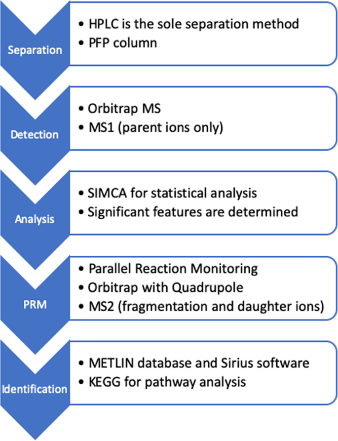
Process scheme for analysis and identification of analytes.
Data processing was performed by initially converting the.raw data files to an mzXML format using the MSconvert software75. The converted files were then imported into the software MZmine 276. Using a Savitzky-Golay filter (5 data point), scan-by-scan filtering was performed on the imported data. A mass peak list was generated using exact mass detection, m/z range of 99–1000 m/z, and mass tolerance of 5.0 ppm. Chromatogram builder settings were: minimum peak height of 10,000 AU and a minimum width of 0.017 min. Deconvolution of these rebuilt chromatograms was performed using a Savitzky-Golay filter with a minimum peak height of 10,000 AU and peak width setting of 0.017–1.0 min. The peak list was filtered using an m/z-range of 99–1000, a retention time range of 0.8–35 min and peak width of 0.017–1.0 min. SIMCA-14 multivariate data processing software was further used to process the peak lists. Principal component analysis (PCA) was performed using Pareto scaling for determination of significant features and to test the statistical fit of the data acquired from sample analysis. Significant features were identified by the METLIN database within a 5 ppm mass tolerance77.
Chromatographic separation and tandem MS analysis were carried out on the QCs of each experimental sample and on a single mixture of standard compounds (100 ppb each) with the use of a high-resolution Q-Exactive Thermo Orbitrap MS (Thermo Fisher Scientific, San Jose, California, USA) operated under the same parameters as described above (same column, methodology, and mobile phases) for samples. MS acquisition was performed through particle reaction monitoring (PRM), with a resolution of 70,000, isolation window of 1.6 m/z, normalized collision energy (dimensionless) of 20 eV and 40 eV, using automatic gain control (AGC) balanced (1,000,000 ions) at 2 Hz. The injection time onto the C-trap was 100 ms. Instrumental settings were: Sheath gas (35 AU), auxiliary gas (5 AU), sweep gas (300 AU), capillary temperature (280 °C), and vaporizer temperature were 35, 5, 300, and 280 °C and the acquisition range was 70–1000 m/z, for the positive and negative ESI methods. External instrument mass calibration was performed every 48 h and was ensured to be within 2 ppm. PRM was carried out on a list of MS1 m/z values that corresponded to all m/z values of VIP > 1, which were determined by the SIMCA software.
As the last step, raw data files of the LC-MS/MS data were imported on MZmine. Chromatograms corresponding to each MS1 m/z on target retention time points were exported as.PRM files. The exported.PRM files were further imported to Sirius 4.0.1 software with settings corresponding to the specific ESI mode and MS2. Feature computations were performed by Sirius using the following software settings: Orbitrap, 5 ppm, 10 candidates, and all PubChem formulas. The predictions of the software were only taken into consideration if at least 3 possible peaks were predicted. A CSI:FingerID search78 was performed and the results were compared with the MS1 METLIN annotations. Additional to the fragmentation pathway analysis, we used the Fragment Similarity function of the METLIN database by inputting the highest 4 peaks on the MS2 chromatograms. In cases where METLIN database’s fragment/daughter ion spectra data were relevant with the groups on MS1-predicted compounds, we chose the compound to be our final annotation. For cases where METLIN database’s fragment prediction was not sufficient, we used the molecular formula prediction of the Sirius software as our final annotation. As examples, the fragmentation mass spectra of parent ions 221.0962, 419.3159, and 440.3575 are given in Figures S4, S6, S8, and the fragmentation trees are given in Figures S5, S7, S9, respectively. In cases where the use of standards of compounds for identification was feasible, we compared the fragmentation patterns of the compounds on their specific retention time points. If the fragmentation patterns were the same, the compound was considered to be verified, and no further analysis of spectra was carried out on METLIN or Sirius.
Determination of compound classifications
Compounds were classified according to their roles in the hydrothermal vent ecosystems. Organosulfur compounds, fatty acids, amino acids, vitamins, nucleosides, and halogenated compounds were reported in different groups. Organic compounds were specified in 4 subgroups based on their elemental structure (CHO, CHOS, CHNO, CHNOS). Furthermore, Van Krevelen plots of elemental ratios of H/C and O/C were plotted to determine the variability of detected organic carbon sources.
Statistical analysis of features by SIMCA
We used SIMCA software for statistical analysis of features determined using the above described method. Principle Components Analysis (PCA), which is a mathematical algorithm that reduces the dimensionality of the data while retaining most of the variation in the data set79, and Orthogonal Projections to Latent Structures Discriminant Analysis (OPLS-DA) statistical processing were used to group samples. It is important to note that OPLS-DA is considered a classed multivariate approach that discriminates separations based on user-defined groups16. It is therefore important to highlight that mild separation between groups was still observed when unclassed principle component analysis (PCA) was performed.
In terms of feature selection, a feature loading S-plot that separates features based on the OPLS-DA separation was first prepared. From this S-plot, features found to separate at the top right and bottom left of the main linear cluster were manually selected and listed in a table. Features in this list were furthered filtered with the use of SIMCA’s proprietary Variable Importance in Projection (VIP) algorithm, where features possessing a VIP >1.000 were deemed significant80. It should be highlighted, however, that VIP has been deemed a “black box” algorithm by some users given that details pertaining to VIP have been kept secret by Umetrics80. Moreover, it has been previously indicated that VIP filtering may unnecessarily remove features that exhibit lower relative signals even if they reveal an absence-presence relationship between 2 samples. Nonetheless, a selection of significant features differentiating the biochemical profiles of two samples extracted by the coated bolts was successfully achieved through the use of the described methodology.
Source: Ecology - nature.com
