Fresh groundwater discharge insignificant for the world’s oceans but important for coastal ecosystems

Modeling coastal groundwater discharge

We simulated submarine and terrestrial groundwater discharge in coastal groundwater systems using a numerical model of coupled density-driven groundwater flow and solute transport. The model code, GroMPy-couple⁵¹, is a Python shell around the finite element code escript^52,53 which has been used previously to simulate subsurface fluid flow⁵². We implemented an iterative scheme⁵⁴ to solve the fluid flow and solute transport equations and the equations of state for fluid density and viscosity. GroMPy-couple uses an implementation of a seepage boundary condition based on an existing implementation in the model code MODFLOW¹⁴, which ensures a realistic and numerically stable partitioning between onshore and offshore groundwater discharge in models of coastal groundwater systems¹⁴. The model code simulates the flow of fresh (meteoric) groundwater, the mixing and recirculation of seawater at the fresh-salt water interface at the coast due to dispersion and the onshore and offshore discharge of groundwater. We did not model transient processes like tidal forcing of groundwater flow and wave setup, that are responsible for the bulk of the recirculation of seawater in coastal aquifers^55,56. Note that the submarine discharge of fresh groundwater is relatively insensitive to transient flow induced by wave set-up and tides⁵⁶. The model code has been validated by comparison with a salt water intrusion experiment⁵⁷ (Supplementary Fig. 9), analytical solutions of groundwater discharge^13,14 (Supplementary Figs. 10, 11), and model experiments using the widely-used model code SUTRA⁵⁸ (Supplementary Fig. 12). See Supplementary Note 1 for more details on the model approach and for more information on the validation of the model code.

Model geometry

Groundwater flow was simulated in a two-dimensional cross section of the subsurface. While we acknowledge that coastal groundwater flow is a three dimensional process, the computational demands of running large numbers of three dimensional models would be prohibitive, given the high spatial resolution required to accurately model density-driven flow and the constraints on timestep size imposed by numerical stability of modeling advective solute transport⁵⁹.

We assigned a constant linear slope to the terrestrial and marine parts of the model domain. The linear slope is a simplification. Testing more complex topographies, with for instance a lower slope of the near-shore parts that is often found in sedimentary settings, or conversely high relief and cliffs in erosional settings would increase the number of model runs that are needed to cover parameter space significantly, and would make the computational costs prohibitive. We therefore aimed to cover the first order effects of a linear topography.

The first 1000 m of the model domain are covered by seawater. The length of the landward size of the model was constrained by the watershed length described elsewhere in the Methods. The thickness of the model domain was kept at 100 m for the exploration of the parameter space, and was varied between 100 and 500 m for sensitivity analysis.

We applied a spatial discretization that varied from 3 m in a zone that extends 500 m offshore and 250 m onshore to 10 m on the landward boundary of the model domain. The zone with fine discretization is centered around the fresh-salt water interface that was calculated using an analytical solution⁶⁰:

where y is the depth of the interface below sea level (m), K is hydraulic conductivity (m s⁻¹), which is calculated as (K = rho _{mathrm{f}}gkappa /mu), ρ_f and ρ_s are the density of freshwater and seawater, respectively (kg m⁻³), Q is the discharge rate of fresh groundwater (m² s⁻¹) and x is distance to the coastline (m). The discharge term (Q) in Eq. (1) was calculated using a depth-integrated version of Darcy’s law:

where b is aquifer thickness (m), and h is hydraulic head (m). In case the calculated discharge exceeded the total recharge volume (i.e., the product of the recharge and length of the model domain) into the system, discharge term Q was capped to equal the recharge volume.

Initial and boundary conditions

A specified recharge flux boundary and a seepage boundary condition were applied to the upper model boundary at the terrestrial side of the model domain. For the seaward side of the model domain we applied a specified pressure that equals the load of the overlying seawater. Initial salinity was equal to seawater values of 0.035 kg kg⁻¹ under the seabed and in a saltwater toe that extends inland following Eq. (1). No flow was allowed over the left-hand and right-hand side of the model domain. Initial pressures were calculated by solving the steady-state version of the groundwater flow equation (Supplementary Note 1 and Eq. (1)).

The exchange of groundwater and surface water or evapotranspiration was simulated using a seepage boundary algorithm¹⁴. The seepage algorithm was chosen because it represents a more realistic upper boundary than often used fixed specified pressure or flux boundaries, while avoiding the computational cost of explicitly modeling evapotranspiration and surface-groundwater exchange. The seepage boundary condition was implemented using an iterative procedure. First, initial pressures were calculated by solving the steady-steady-state version of the groundwater flow equation, i.e., the groundwater flow equation with the derivative of pressure and concentration over time set to zero. For the first step a specified flux was assigned to the entire top boundary, which represents groundwater recharge from precipitation. Following the first iteration step, a specified pressure boundary was adopted at any surface node where the fluid pressure (P) exceeds 0 Pa. Fluid pressures were then recalculated again by solving the groundwater flow equation using this new boundary condition. Following each iteration step, the flux to the boundary nodes was calculated by solving the steady-state groundwater flow equation. Any surface nodes where the fluid pressure exceeds 0 Pa are added to the seepage boundary and are assigned a specified pressure of 0 Pa. Seepage boundary nodes that instead of outflow generate inflow into the model domain at a rate that exceeds the recharge rate were removed from the seepage boundary. To avoid oscillations in the solution, only the nodes that generate 10% or more inflow compared to the seepage node with the highest rate of inflow are removed from the boundary condition after each iteration. This iterative procedure is continued until the number of seepage nodes reaches a steady value.

The iteratively calibrated steady-state seepage boundary is used as an initial seepage boundary during the transient model runs. At each timestep, the active seepage boundary is inherited from the previous time step. The seepage boundary condition is removed for any node that has become a net source of water into the model domain. Any non-seepage node at the surface where the fluid pressure exceeds 0 Pa is added to the seepage boundary. This implementation of the seepage boundary condition ensures that the hydraulic head never exceeds the surface elevation, and that there is not more inflow than the specified recharge rate at any node at the surface. Both possibilities would be unrealistic, but allowed when either a specified flux or a specified pressure boundary condition would be used for the upper boundary. In addition, the seepage boundary method as implemented here avoids the use of an unknown and uncertain drain conductance parameter that is used in drain boundary conditions, which aim to provide a similar realistic upper boundary as the seepage boundary¹⁴ but use a different algorithm to achieve this.

Assumption of constant thickness and saturation

The model domain was assumed to be fully saturated and the saturated thickness was constant in the model domain and independent of the modeled pressures and hydraulic head. This is a simplification that avoids the numerical instability and high computational costs of modeling unsaturated groundwater flow in combination with density-driven flow. At the same time, it makes comparisons between the individual model runs easier, because saturated thickness and transmissivity remain constant unless permeability is changed. In addition, when not adopted, the modeled thickness of the model domains for the different model scenarios would have to be sufficiently high to accommodate all possible modeled hydraulic gradients, which vary from values close to the highest modeled topographic gradients to values of near zero for the different model scenarios. This would again result in a prohibitively high number of model runs that would be required to cover the range found in coastal groundwater systems.

The assumption of a fully saturated subsurface does introduce errors in the modeled flow field. For models with a high topographic gradient there is a significant vertical flow component in our model setup, regardless of the shape of the watertable and the hydraulic gradient. However, for cases where permeability is high, the hydraulic gradient would relatively low and groundwater flow would in reality be nearly horizontal. The error in the partitioning between horizontal and vertical components of the flow vectors is expected to be equal in magnitude to the difference in topographic gradient and the modeled hydraulic gradient. The median difference between topographic and watertable gradient is 0.17%, and exceeds 5% in 2381 of the 40,082 modeled watersheds. This error however reduces to near zero close to the shoreline, where in all model experiments the watertable was located at or very close to the surface, and where therefore the assumption of fully saturated conditions is correct. Given the fact that the near-shore part of the model domain is by far the most critical for our model results on submarine and near-shore groundwater discharge, we expect the assumption of fully saturated conditions to not significantly influence the results reported here.

We used a constant thickness over the model domain. The thickness was varied between 50 and 500 m in a first sensitivity analysis. For the final model runs we adopted a standard thickness of 100 m, which is equal to the median aquifer thickness that were used to compile data for a global permeability map²², and is roughly equal to the thickness where the majority of young groundwater and active groundwater circulates following global compilations of radiogenic isotope data of groundwater^15,16. Adopting a standard thickness of 100 m ensures that the modeled values of transmissivity (the product of permeability and thickness) are consistent with the global permeability map.

Model runtime

The transient models were run until a steady state was reached. We assumed that the model has reached steady state when the change in pressure is less than 1 Pa a⁻¹ and the change in solute concentration that is less than 1 × 10⁻⁴ kg kg⁻¹ a⁻¹. The initial timestep size was 5 days and was increased by a factor of 1.03 after completing each timestep. To avoid numerical instability in solving advective solute transport, the maximum size of the timestep was adjusted automatically to not exceed the Courant-Friedrichs-Lewy (CFL) condition⁶¹:

where q is fluid flux (m s⁻¹), Δt is timestep size (s) and Δx is the size of one element (m) as calculated by escript⁵³. We used a relatively low limiting value of CFL = 1.0 to ensure numerical stability for the large set of different models that we tested.

Model sensitivity analysis and exploration of parameter space

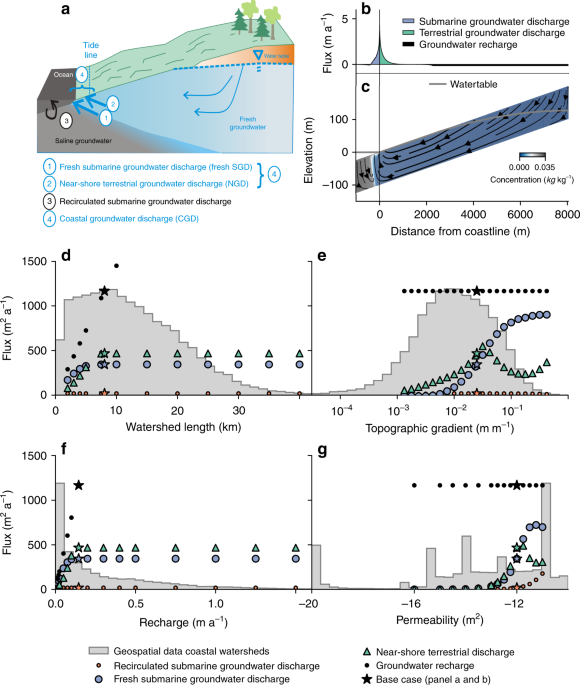
First, we performed a sensitivity analysis of submarine groundwater discharge by varying watershed length, topographic gradient, groundwater recharge and permeability in a range covers the values found in the geospatial analysis (Supplementary Fig. 2; Supplementary Table 3). The sensitivity analysis consisted of a total of 130 model runs. The parameters ranges are shown in Supplementary Table 4. The base case model used the median watershed length and groundwater recharge from the geospatial analysis, and a higher permeability (10⁻¹² m²) and topographic gradient (2.5%) than the median watershed to better show the sensitivity of coastal groundwater discharge to the various parameters. In addition to the results shown in Fig. 1 we tested the effect of a realistic range of values of aquifer thickness, permeability anisotropy, and longitudinal dispersivity, which are variables for which no geospatial data was available. These additional results are shown in Supplementary Fig. 13 and discussed in Supplementary Note 2 and confirm that although these parameters are important, permeability and topographic gradient are by far the most sensitive parameters for coastal groundwater discharge.

Second, we conducted a number of model experiments (n = 495) to explore the parameter space for recharge volume (recharge multiplied by contributing area), topographic gradient and permeability. The ranges of these parameters are shown in Supplementary Table 5. The length of the model domain was kept constant at 3 km in all these model runs to reduce the number of runs require to cover parameter space. This does not affect model results because the model sensitivity analysis shows that changes in recharge volume by either changing the contributing area (watershed length) or the groundwater recharge rate have the same effect on modeled groundwater flow and discharge (see Fig. 1d, f). Apart from the recharge volume, permeability, and topographic gradient all other parameters were constant and followed the base case values listed in Supplementary Table 5. A number of runs (n = 144) did not converge to steady-state after a total number of 10,000 timesteps or were numerically unstable and were discarded. These consisted predominantly of models with a very low topographic gradient (<10⁻³ m m⁻¹) or recharge rate (<0.01 m a⁻¹), where flow rates were so low that numerical precision affected the results.

Longitudinal dispersivity was kept constant at a value of 50 m and transverse dispersivity was assumed to be 0.1 times longitudinal dispersivity. Compilations of dispersivity data suggests that for the scales of the numerical models presented here longitudinal dispersivity varies between approximately 10 and 100 m, while transverse dispersivity is an order of magnitude lower⁶². However, some case studies in coastal aquifers have reported much lower numbers⁶³. Nonetheless we have opted to use relatively high values of longitudinal and transverse dispersivity of 50 and 5 m, respectively. The reason is that lower values would strongly increase the computational costs, since for lower values of dispersivity one would have to decrease the grid cell size and increase the number of grid cells. Sensitivity analysis confirm that at least for values of longitudinal dispersivity of 50 m or more coastal groundwater discharge is relatively insensitive to dispersivity (Supplementary Fig. 13).

Permeability anisotropy (the ratio of horizontal over vertical permeability) was kept constant at a value of 10. For fractured crystalline rocks vertical permeability may exceed horizontal permeability, whereas for layered sediment sequences anisotropy can reach a factor of 100 or more⁶⁴. We used a constant anisotropy value of 10 to strike a balance between these two end-members. Note that a more accurate implementation of permeability anisotropy in our models would require information on the orientations of fractures and bedding in coastal aquifers, which are currently not available at a global scale.

Geospatial data analysis

The model input was based on a geospatial data analysis of the controlling parameters of coastal groundwater discharge. We analyzed watershed geometry⁶⁵, topographic gradients⁶⁶, permeability²², and groundwater recharge^23,24 for 40,082 coastal watersheds globally (see Supplementary Fig. 2).

Watershed geometry

We used the geometry of coastal watersheds as a first order estimate of the size coastal groundwater systems. Note that in our model setup the area contributing to coastal discharge is determined by the model itself and the seepage boundary condition, and depends on the flow capacity of the subsurface and the recharge volume. In areas with high permeability, high relief, or low recharge the watertable can be decoupled from topography and regional flow that bypasses the nearest discharge points can be significant^67,68, which means the contributing area could be larger than the size of the model domain. A published comparison of recharge and discharge estimates in a large number of river basins indicates that for the majority of basins the regional flow component is less than 50%⁶⁹. To cover the uncertainty of the size of the contributing area in our calculations of coastal groundwater discharge, we used a value of two times the size of surface watersheds as a maximum estimate.

First, 40,082 coastal watersheds were selected using global watershed⁶⁵ and coastline⁷⁰ datasets. Second, the local watershed divide to the ocean for each watershed was identified using GIS tools. The local watershed divide was defined as the boundary between each watershed and adjacent non-coastal watersheds. The representative length scale was taken as the mean distance of the water divide to the coastline. For watersheds that were only bound by other coastal watersheds we used the mean distance of the centroid of the watershed to the coastline as a representative length scale. Note that the global analysis may underestimate coastal groundwater discharge in several tropical islands in the Pacific, since islands such as Hawaii and Mauritius are missing from the global watershed database⁶⁵ that supports the analysis.

Permeability

Permeability of each coastal watershed was extracted from a global dataset of near-surface permeability (up to ~100 m depth)²². The permeability map is based on a high-resolution global map of surface lithology⁷¹ and a compilation of large-scale permeability estimates of near-surface geological units²². We made two changes compared to the permeability map with the aim of ensuring that the modeled coastal groundwater discharge is a high, but still conservative and realistic estimate.

In the global permeability map, areas in which the lithology consisted of mixed unconsolidated sediment or unconsolidated sediments with an unknown grain size were assigned a relatively low permeability (10⁻¹³ m²)²². This value is below the threshold for generating significant coastal groundwater discharge, except for settings with a very high topographic gradient. However the multimodal distribution of this unit²² suggests that in many cases this unit contains coarse grained sediments. In layered unconsolidated sediments, the effective permeability is likely to be close to the value of the most permeable sub-unit, whereas the permeability value assigned in the global permeability map is the mean permeability on a log scale. We instead assume that the permeability for coarse-grained unconsolidated sediments (10^−10.9 m²) is more appropriate to simulate regional groundwater flow in coastal aquifers that were classified as mixed or unknown unconsolidated sediments in the global permeability map.

The permeability of carbonates in the global permeability map is likely underestimated in coastal areas with strong karstification. Coastal carbonates are predominantly karstified⁷², in part because the fresh-salt water mixing zone at the coastline promotes dissolution and the formation of permeable karst conduits⁷³. We therefore adopted a higher permeability estimate equal to the value reported in the global permeability map plus one standard deviation (10^−10.3 m²). While we acknowledge that this value is highly uncertain as a global average for coastal karst aquifers, and that in reality their permeability is likely to be highly variable, this value is in line with reported values of regional-scale permeability in coastal karst aquifers^74,75,76.

Topography

Elevation data⁶⁶ was extracted for each coastal watershed. We calculated distance to the coastline and elevation for each point in the elevation raster. We then calculated the average and standard deviation of the topographic gradient by dividing elevation by the distance to the coast. In addition, we calculated the topographic gradient for raster cells that contained a stream. The locations of streams were obtained by grouping raster cells for which the distance to the coast is the same within a range that is equal to the size of one raster cell, and then selected the raster cell with the lowest elevation for each distance value.

Additional geospatial datasets

We extracted a number of global datasets for a comparison with the calculated submarine and terrestrial discharge, including river discharge²³, potential evapotranspiration²⁷, the elevation of tide and storm surges⁷⁷, and watertable gradient, which was quantified using a global model of watertable depth⁷⁸ and global elevation datasets⁶⁶.

Representative topographic gradient

The numerical models used for the model sensitivity analysis and the global estimate of coastal discharge use a linear topographic gradient. The topographic gradient is important because it sets a maximum for the hydraulic gradient in each watershed and because it governs the partitioning of coastal groundwater discharge between NGD and fresh SGD (Fig. 1e). We explored which metric can be used as a representative linear topographic gradient by comparing coastal discharge for a series of model runs that include into account the real topography with cross-sectional groundwater models that only include a linear topography. An example comparison of these two model approaches for a watershed is shown in Supplementary Fig. 14. The comparison shows that for most of the tested watersheds coastal groundwater discharge can be represented by cross-sectional models that use the average topographic gradient of an entire watershed, or the average topographic gradient of stream channels in each watershed (Supplementary Fig. 15). See Supplementary Note 3 for more details on these model experiments. Based on these results we used the average topographic gradients in coastal watersheds as a best estimate in further model experiments and the average topographic gradient of streams as a lower bound for the uncertainty range of coastal groundwater discharge.

Quantification of global coastal groundwater discharge flux

Global fluxes of CGD, fresh SGD, and NGD were obtained by linear interpolation of 351 model results to the 40,082 coastal watersheds (see Fig. 2 and Supplementary Figs. 3, 4). The interpolation is based on a comparison of permeability, topographic gradient, and recharge volume, which is the product of groundwater recharge and the size of the contributing area, for the model results and the geospatial data of coastal watersheds. For each watershed CGD was calculated by linear interpolation of the modeled CGD values of the model runs with the closest values of recharge volume, permeability and topographic gradient. A comparison of the modeled and interpolated values of CGD is show in Fig. 2. For n = 13,025 watersheds the parameter values were located outside the bounds of the parameter combinations tested by the model runs. These were predominantly watersheds with in which permeability was lower than the lowest modeled permeability value (<10⁻¹⁶ m²). In these cases we used a nearest neighbor algorithm⁷⁹ to assign the CGD value of the closest model run to the watershed. The average difference between linear interpolated and the nearest modeled CGD value in log units was 0.26. We repeated the same interpolation procedure to calculate fresh SGD (Supplementary Fig. 3), NGD (Supplementary Fig. 4), maximum discharge flux and the horizontal and vertical extent of the submarine and terrestrial discharge zone for each coastal watershed.

We used reported ±1 standard deviation uncertainty of permeability²², the differences between two alternative recharge datasets^23,24 and the differences in the topographic gradients between elevation grid nodes covered by streams and the entire coastal watershed to calculate minimum and maximum estimates of the discharge fluxes. The interpolation yielded two dimensional cross-sectional fluxes in units of m² a⁻¹. Volumetric fluxes were calculated by multiplying the flux by the length of the coastline for each watershed. While the coastline length is in principle a fractal property with a value that depends on the scale of observation, in our case a value was chosen such that the product of the coastline length and the representative length scale of each watershed equaled the area of each watershed. The interpolated values of groundwater discharge were compared to published values of surface runoff²³, potential evapotranspiration²⁷, groundwater depletion⁴⁵, and tide and storm surge elevation⁷⁷, which were assigned to each watershed using GIS tools. For the comparison of the spatial distribution of CGD and runoff, evapotranspiration or depletion, all fluxes were summed up at the watershed scale.

Model-data comparison

Comparison between modeled and measured average hydraulic gradients in 336 coastal watersheds with water level observations from a global dataset⁷⁸ shows that the ratio of the modeled values over the measured values is 1.08 (see Supplementary Note 4 and Supplementary Fig. 6) when using the best estimates of permeability, recharge, and topographic gradients. This shows that the model provides a realistic estimate of coastal groundwater flow. Overall ~60% of the local variability in water table gradient is captured. The remaining variation is likely due to the large spatial scale of our models (on average 11 km) and the limitations of the global datasets supporting our analysis. A qualitative comparison with locations of reported ecosystem impacts by fresh SGD and reported use of fresh SGD shows that in all of these locations the modeled fresh SGD is much higher than the median of all coastal watersheds globally (see Supplementary Tables 1, 2). Comparison to a selection of ten published local estimates of fresh SGD shows that for five studies the modeled and reported fresh SGD values fit within uncertainty bounds (Supplementary Fig. 16a; Supplementary Table 6). However, for the remaining locations the reported values strongly exceed the modeled values, but the reported fresh SGD also exceeds the total groundwater recharge in adjacent coastal watersheds (Supplementary Fig. 16b). This in spite of the fact that all of the reported values are located in watersheds with perennial streams that also discharge a large part of the overall groundwater recharge. This suggests that these studies strongly overestimate fresh SGD. The frequent inconsistency of fresh SGD estimates with onshore groundwater budgets has been noted earlier by several authors^11,80 and may be due to uncertainties in methods to quantify fresh water discharge^81,82 or biased selection and reporting of study sites for SGD¹.

Quantification of solute transport

First-order estimates of the global solute flux that is transported by fresh SGD were calculated by multiplying the calculated global fresh SGD flux with previously reported average values for the concentrations of nitrogen^28,29, carbon⁸³, silica⁷, and strontium⁸ in coastal groundwater. These estimates were compared to published values of the solute flux by surface runoff and earlier estimates of the contribution of fresh SGD^7,8,30,83. These estimates are based on published compilations of data predominantly from the US, which we consider as first order estimates for concentrations in groundwater at a global scale that are relatively uncertain. The estimate of carbon was based on the global average DIC in soil water of 15 mg L⁻¹ as calculated from reported global DIC fluxes to the groundwater table and groundwater recharge by Kessler and Harvey⁸⁴. The average strontium concentration in groundwater of 2.9 μM reported by Beck et al.⁸ is based on compilations of groundwater strontium data and an extrapolation based on a global lithology map. The nitrogen concentration of 2 mg L⁻¹ was based on a reported median value for a large dataset from the US³⁹. The silica concentration was equal to a value reported by Frings et al.⁸⁵ based on a compilation of groundwater data predominantly from the USA. The calculated values of the global solute flux by SGD were compared to published values of the solute flux by surface runoff and earlier estimates of the contribution of fresh SGD^7,8,30,83. Note that our estimates assume conservative transport and do not take into account fluid-rock interaction and microbial activity in coastal aquifers. Several studies have shown that intensive reactions happen in the mixing zone between fresh-and saltwater (subterranean estuary). Despite the effects that were described for individual local systems, no large scale estimates of the effect of subterranean estuaries are known to the authors, therefore this effect cannot be quantified in this study.

Estimation of eutrophication risk

The risk of eutrophication of coastal ecosystems was estimated by comparing locations of high groundwater discharge with high agricultural nitrogen inputs in coastal watersheds. Areas with high risk were identified if CGD exceeded a threshold of 100 m² a⁻¹ and nitrogen inputs⁸⁶ exceed 10 kg ha⁻¹. The threshold value for CGD is based on a review of locations with reported impacts of coastal groundwater discharge on ecosystems (see Supplementary Note 4 and Supplementary Table 7). The threshold value for nitrogen input corresponds to values that have historically led to strongly elevated nitrogen concentrations in groundwater in Europe and North America^39,40 that have contributed to the eutrophication of terrestrial and nearshore ecosystems⁴¹. Given the very high sensitivity of coastal ecosystems and especially coral reefs to nitrogen⁸⁷, this threshold value is likely to result in a relatively conservative estimate of eutrophication risk. The calculated locations of sites with high eutrophication risk was compared with the location of sensitive ecosystems such as estuaries⁴², salt marshes⁴³, and coral reefs⁴⁴. We acknowledge that eutrophication of marine ecosystems is a complex function of nutrient input, transport, denitrification, and mixing with seawater. The eutrophication risk reported here should be considered as a first order estimate that can guide follow-up studies. Finally we also compared the modeled coastal groundwater discharge fluxes to groundwater depletion by using published groundwater depletion rates⁴⁵ and multiplying these rates with the area of coastal watersheds.