Mosquito mass rearing
To achieve stable production of males, we developed an automated larval rearing system (LRS) that takes first instar larvae as input, and outputs pupae (Fig. 2a). Prior to loading onto the LRS, eggs are hatched overnight, after which L1 larvae are automatically counted using a COPAS 550 (Union Biometrica) large-particle flow cytometer into 50-ml conical tubes. The first step in the LRS is larval container assembly, in which disposable plastic containers are filled with water and food. Larvae are automatically transferred from the conical tube into the container by a robotic larval transfer arm. After filling and sealing, containers are automatically transferred to an incubated storage and retrieval frame (Supplementary Video 1). Larvae develop for 6 days in the frame, during which they are automatically fed. On the seventh day most larvae have developed into pupae and the containers are removed from the frame to be sex sorted (Supplementary Video 1). At maximum capacity and high rearing density, the LRS is capable of producing over 2,950,000 male pupae per week.
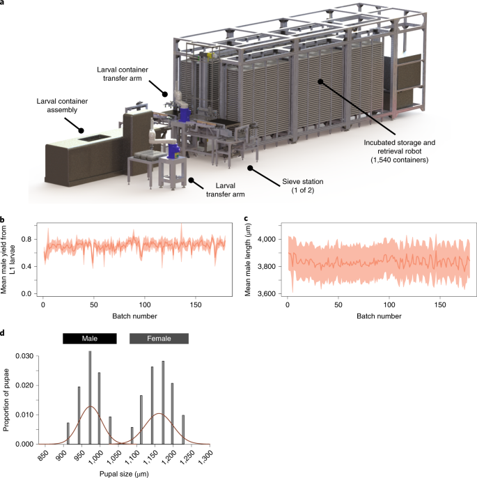
a, Schematic of the LRS with major components labeled. b, Optimized rearing protocols resulted in a highly consistent yield, calculated as the ratio of adult males entering the release tubes relative to the number of L1 larvae introduced into larval containers. The dark line shows mean yield, shading represents the s.d., the x axis represents all 2018 production batches (n = mean of 96, range of 10–140 independent sex-sorter measurements per batch). c, Consistent mean length of adult males as measured from sex-sorter images (s.d. interval shaded, n = mean of 43,256, range of 5,827–64,282 independent male length measurements per batch). d, Discrete pupal size dimorphism between sexes. Histogram shows width estimates from ~18,000 pupae. Pupal width is measured in pixels resulting in bins when converted to μm. Red lines show normal distribution fit to male and female sets separately.
The LRS produced remarkably consistent numbers of synchronous, similarly sized pupae from each rearing container. To visualize the consistency of production, we calculated the daily yield of male mosquitoes over 179 production batches during our 2018 field trial. Yield was calculated as the proportion of L1 male larvae that developed into adult males and passed through the visual sex-sorting pipeline (see below). The LRS showed high temporal consistency with an average yield of 70.39% (Fig. 2b). In addition, adult male size, estimated from the body length of male mosquitoes, was also highly consistent throughout the 6 months of production, averaging 3.8 mm (σ2 = 0.9 mm; Fig. 2c). A. aegypti is sexually dimorphic for pupal size under favorable conditions38. Our rearing protocols (Supplementary Text) implemented on the LRS produced consistent pupal sizes resulting in clear separation between the sexes, with female pupae on average 19.26% larger than male pupae (Fig. 2d), consistent with optimized larval development39.
Mosquito sex sorting
To minimize the chances of unintentional female release, we developed an automated, multi-step sex separation process based on known morphological differences between males and females (Fig. 3a). The first step is an automated mechanical sieve that separates based on body size, allowing male pupae to pass through while females are retained. Over the course of 2018 production, an average of 2.54% of pupae that passed through the sieve were females. Assuming a 50/50 input pupal sex ratio, we estimated that automated mechanical sieving removed 94.92% of females (Fig. 3b).
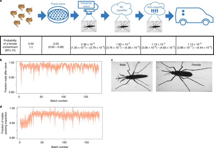
a, Illustration of the entire sex-sorting pipeline, including the mechanical pupal sieve, real-time adult visual inspection, cloud-based machine learning classifier, and non-expert review. The probability of a female contaminant with 95% CIs for each step is shown along with the estimated overall female contamination rate for the entire pipeline in the final column. b, The fraction of mosquitoes imaged by the sex sorter after the pupal sieve that were male with s.d. intervals shaded for 179 production batches. c, Example images from the adult sex sorter (male on the left and female on the right) used by both the industrial vision system and machine learning classifier. d, The fraction of true males that were correctly labeled and accepted by the Industrial Vision system with s.d. interval shaded (n = mean of 96, range of 10–140 independent sex-sorter lane measurements per batch).
In the second step, the primarily male pupae that passed through the sieve are loaded onto a real-time visual sex-sorter where they eclose and — of their own volition — walk down a narrow path over which a camera is mounted (Supplementary Video 2). Custom industrial vision software recognizes each ambulatory mosquito as an object, attempts to physically isolate them using air jets and a shutter, and then takes at least one image. If multiple mosquitoes make it into the imaging area they are always rejected. Images with a single mosquito are inspected for male-specific body parts (Fig. 3c), including genitalia and antennal features, using a template matching algorithm. Individuals with male morphology are puffed into a container used to distribute mosquitoes in the field, called a ‘release tube’, while individuals failing inspection are rejected. At the start of the 2018 field season, an average of 89.85% of males passed inspection (Fig. 3d). After implementing improved traffic management algorithms to better isolate individuals, 95.59% of males passed inspection, resulting in consistently high male yield through the adult sex sorters.
In the third step, we submit all images of individuals labeled male by the industrial vision system for scoring by a machine learning classifier. The classifier is a deep neural network built upon the open source Inception-v3 architecture40 and trained using 2.1 million manually labeled images. The classifier computes the probability that the individual is male and the images are ranked based on their maleness score, subsampled, and sent to a panel of five trained, but non-expert, reviewers via an online micro-task platform for inspection and labeling. We sent two samples for review: the 1% of images with the lowest male probability, and a 1% random sample of all male images. If the non-experts identified a female or if there was any inconsistency in their labels, an expert reviewed the images in question. If the expert confirmed any females, we located and purged the part of the release tube with the female before the tube left the factory.
Based on data from 2018, we estimated the probability of a female contaminant at each step of the sex-sorting pipeline (Fig. 3a). Assuming independence between the different steps in the pipeline, the combined system is expected to release 1 female for every 900 million males with a 95% CI of 1:200 million to 1:26 billion (Fig. 3a and Supplementary Text). For additional validation of the sex-sorting pipeline, we screened larvae obtained from ovitraps in our treatment areas and found no Wolbachia-positive larvae (Supplementary Text), confirming that we did not unintentionally establish a Wolbachia-infected population in the field as would be expected if we released infected females into an area in which the wild-type population had been suppressed.
Automated male mosquito releases
For a SIT intervention to be successful, released males must permeate the landscape to find unmated females. We developed an automated male mosquito release system to ensure complete and calibrated distribution of Wolbachia-infected males into treatment areas. The system includes transport and release tubes, automated release devices mounted inside customized vans (Fig. 4a), map-based release plan generation and triggering software (Fig. 4b), and a structured light mosquito counter (Supplementary Text).
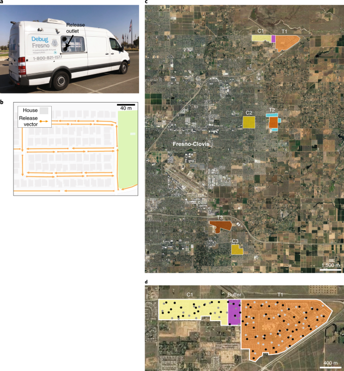
a, Wolbachia-infected males were released into field sites using two sprinter vans equipped with automated release devices that blew males through release outlets on the rear passenger side. b, Release map indicating a planned route for van drivers to follow, triggering the release device. Each orange vector indicates the GPS location and direction of travel at which a segment of the release tube was released. c, Map of treatment areas (T1–T3) in shades of orange and control areas (C1–C3) in shades of yellow. The C1 control buffer area is shaded in purple, and the T2 treatment buffer is shaded in turquoise. These areas were monitored but not included in analysis. Only the T2 treatment buffer was treated with sterile males. d, Representative placement and density of adult BG-Sentinel traps (black dots) and egg traps (gray dots). Trap density was similar between treatment and control areas (Supplementary Table 1).
After a preliminary study in 2017 (see Supplementary Text for details), starting on 16 April 2018 we conducted daily releases of Wolbachia-infected A. aegypti males over a period of 26 weeks into 3 treatment sites (labelled T1, T2, and T3 in Fig. 4c), which include 3,063 households across 293 ha (Supplementary Table 1). These sites were residential neighborhoods typical of the area, situated on the edge of the Fresno-Clovis metropolitan area with at least partial isolation, and were known to have established A. aegypti populations based on historical trapping data. We measured adult mosquito density using BG-Sentinel traps (V2, Biogents) placed at comparable densities in both treatment and control sites (Fig. 4d and Supplementary Table 1).
In 2018, we released Wolbachia-males at an average rate of 78,469 per day or 267.81 (σ = 61.16) males per hectare per day for a total of 14,376,511 male mosquitoes during the study, although release rates differed between sites according to both household counts and the number of females in traps in each site (Fig. 5a–c and Supplementary Table 2). We also varied release rates per site within the three study phases. In phase I (mid-April to mid-May), release numbers were determined exclusively by the number of households in each site. In phase II (mid-May to late July), we increased the number of males per household for treatment sites T2 and T3, as historical data indicated that these sites have had higher wild mosquito densities and are less geographically isolated than T1. In phase III (late July to mid-October), we held the release numbers constant for sites T2 and T3, but reduced the T1 release rate in response to our monitoring data, which indicated very high ratios of Wolbachia-infected to wild-type males in this site (Supplementary Table 3). We monitored male mosquito densities using adult mosquito traps and found that male mosquito numbers reflected the different phases of release (Fig. 5b).
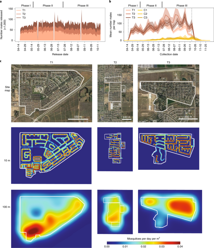
a, Stacked sum plot showing the total number of males released into each treatment area over the 6-month study period (see the main text for a description of study phases). We released males every day, except for three pauses for US holidays. b, Mean number of adult males per trap in treatment areas (T1–T3) and control areas (C1–C3) with 95% bootstrap CIs (nT1 = 44, nT2 = 24, nT3 = 35, nC1 = 17, nC2 = 28, nC3 = 15 independent trap samples per collection day). Dotted lines indicate the first and last day of releases. c, Top, satellite maps with treatment areas outlined in white and treatment buffers indicated with B in T2. Middle, density of Wolbachia-males, as measured by the onboard structured light mosquito counter, averaged over 6 months of releases assuming a 10-m dispersal kernel revealing van path and variable release rate based on house density. Bottom, density of Wolbachia-males averaged over 6 months of releases assuming a 100-m dispersal kernel, suggesting nearly complete coverage of release areas.
We visualized the density of released males in each neighborhood over the entire 2018 season using data from the van-mounted release device and mosquito counter. First, we modeled the density of released males assuming a 10-m dispersion kernel around GPS (global positioning system) release coordinates, which shows the van release route and highlights variations in release rate due to changes in housing density (Fig. 5c). Importantly, if we assume a more realistic dispersion kernel of 100 m, males are more evenly distributed across each site, suggesting comprehensive coverage. The only two relatively low-density spots (blue regions) correspond to a large elementary school in the center of T1 and a low-housing-density section of T3 (Fig. 5c). To evaluate the precision of releases, we compared our intended mosquito distribution targets (based on housing density) to a map of actual mosquito release density assuming a 100-m male dispersal kernel. The density of male distribution after releases largely matches the intended distribution and captures the reduction and increase in release rates in T1 and T3, respectively (Supplementary Fig. 1).
Suppression of mosquito populations in release sites
The goal of field releases was to test whether a high ratio of Wolbachia-infected males to wild-type males would result in enough incompatible matings to sharply reduce egg hatch and subsequently the wild-type adult population. To best isolate the effect of the Wolbachia-male releases, only normal mosquito abatement activity under the mandate of the California Mosquito Abatement District (CMAD) was applied in the treatment and control areas (Supplementary Table 4 and Supplementary Text).
We monitored the ratio of released to wild-type males (that is, overflooding ratio) by testing trapped adult males for Wolbachia using a loop-mediated isothermal amplification (LAMP) assay (Supplementary Text) and found that our releases resulted in high overflooding ratios in each of the treatment sites during the first 4 months of release, ranging from 47.53 to 557.00 (Supplementary Table 3). As overflooding ratios reached levels too high to be estimated reliably, we did not measure these for the last 2 months of releases. The overflooding ratios tended to increase month after month, consistent with both increased release rates in T2 and T3 during phase II and declines in the number of wild-type males per trap (Supplementary Table 3).
We also monitored the abundance of adult females using BG-Sentinel traps (Fig. 4d) and found that the density of adult females differed significantly between treatment and control areas during the treatment period. In each control area, the average number of females per trap night followed the expected seasonal curve, with the population increasing in June, peaking from July to September with female densities of >12 females per trap in each site, and declining in October (Fig. 6a). In contrast, female abundance in the treatment sites had a strikingly different pattern (Fig. 6a,b). T1, the most isolated site, had extremely low numbers of females in all weeks, peaking at an average of only 0.6 females per trap in the third week of October. Although sites T2 and T3 had more females than T1 as the season progressed, with peak mean females per trap of 1.52 and 2.17, respectively, the 95% confidence intervals (CIs) are fully separated from those of the control sites from mid-July to mid-November (Fig. 6a).
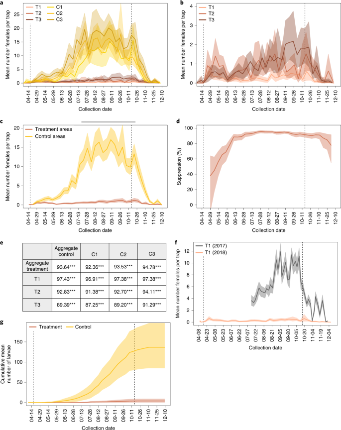
a, Mean number of females per trap in treatment areas (T1–T3) and control areas (C1–C3) in 2018 (nT1 = 44, nT2 = 24, nT3 = 35, nC1 = 17, nC2 = 28, nC3 = 15 independent trap samples per collection day). b, Mean number of females per trap in treatment areas only, on shortened y axis (sample sizes are the same as in a). c, Mean number of females per trap for aggregated treatments sites and aggregated control sites (nTRT = 103, nCTRL = 60 independent trap samples per collection week). Gray bar, period defined as ‘peak season’. d, Per cent suppression of adult females in aggregate treatment sites compared to aggregate control sites using a 2-week trailing average (see Supplementary Text for details; sample sizes are the same as in c). e, Suppression calculated across the 14-week peak-season window evaluated with a one-sided permutation test (nT1 = 616, nT2 = 336, nT3 = 490, nC1 = 238, nC2 = 392, nC3 = 210, nTRT = 1,442, nCTRL = 840 independent trap samples). ***P < 1.6 × 10⁻⁵, Bonferroni-corrected. f, Year-on-year comparison of the average number of females in T1; comparison of the same period in 2018 and in 2017 (n2017 = 65, n2018 = 44 independent trap samples per collection day). g, Cumulative mean number of larvae per egg trap with treatment sites aggregated and control sites aggregated (nTRT = 131, nCTRL = 77 independent trap samples per collection week), indicating significantly different larval production between treatment and control areas. For all panels, shaded areas indicate 95% CIs, and dotted lines indicate first and last day of releases.
When comparing female abundance between aggregated treatment and control sites, there is a clear separation between the 95% CIs beginning approximately 5 weeks after the start of releases (Fig. 6c). The average number of females in aggregated treatment sites remained low for the entirety of the season with less than one female per trap night in 32 out of 36 weekly collections and a peak value of 1.2 females per trap night (95% CI, 0.78–2.47) in the third week of October. In comparison, the control sites reached a peak of 16.6 females per trap (95% CI, 13.70–19.87) in the second week of September (Fig. 6c).
Overall, release of Wolbachia-infected males into treatment areas resulted in 93.64% (corrected P = 1.6 × 10⁻⁵) suppression of females from mid-July until the seasonal declines starting in mid-October, with a maximum 2-week suppression level of 95.5% (95% CI, 93.6–96.9%) in the fourth week of July (Fig. 6d). To test the generality of these results, we compared each treatment site individually to both the aggregate and individual control sites and found that significant suppression was achieved in all sites across the 14 weeks of peak mosquito season in all pairwise comparisons (Fig. 6e). Moreover, we found that, within 2-week windows, T1 reached a peak suppression of 98.9% (95% CI, 98.1–99.4), T2 reached 94.8% (95% CI, 92.3–96.8), and T3 reached 94.6% (95% CI, 92.0–96.4) compared to the aggregate control site. Results are similar when each treatment site is compared to individual control sites (Supplementary Table 5). We also compared female abundance in T1 in 2018 with that in 2017 (Fig. 6f and Supplementary Text), which showed a 97.1% drop in the number of mosquitoes from 2017 to 2018 (95% CI, 95.4–98.6).
Comparison of the number of larvae hatching from egg traps in treatment sites relative to control sites provides an additional view of the effect of Wolbachia-male releases on mosquito reproduction. We directly monitored larval production using egg traps distributed at comparable densities in both treatment and control sites (see Methods, Fig. 4d and Supplementary Table 1). For the entire season, the mean number of cumulative larvae collected per egg trap in treatment sites was 3.7 (95% CI, 0.5–8.4) compared to 126.3 (95% CI, 80.3–180.7) in control sites — a 97.1% reduction in collected larvae (Fig. 6g). Similarly, the mean number of eggs per trap was consistently lower in the treatment areas than in control areas (Supplementary Fig. 2). To infer the proportion of incompatible versus wild-type matings, we also calculated hatch rates of collected eggs. Although variable owing to small sample size, hatch rates of eggs collected in treatment sites were consistently lower than those collected from control areas (Supplementary Fig. 3). Taken together, the data demonstrate that Wolbachia-infected males inhibited mosquito reproduction, resulting in strong suppression of the wild population in release sites.
Mosquito migration into release sites
Despite treatment site selection intended to minimize migration through geographic isolation and treated buffer areas, several lines of evidence suggest that immigration of inseminated females from nearby untreated areas put an upper limit on achievable suppression. Although statistical support is limited by small sample sizes, more females were caught in traps on the outer edge of treatment sites (T2 and T3), as indicated by a negative correlation between the distance of a trap from the edge of the site and the average number of females it collected, whereas only one of the control sites (C2) showed this pattern (Fig. 7a–c and Supplementary Table 6). In addition, we used the LAMP assay to test for Wolbachia-infected males in traps from the buffer area separating T1 and C1 as well as traps within C1 (Fig. 4d). Unsurprisingly, we found Wolbachia-positive males in large numbers up to 200 m from the nearest release street in T1 (Fig. 7d), clearly demonstrating that our treatment sites were within the flight range of mosquitoes in untreated areas. Overall, the data are consistent with ‘edge effects’ driven by female mosquito migration into our treatment sites.
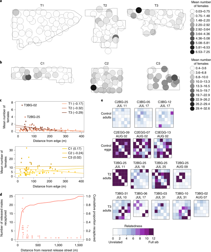
a, Maps of treatment areas with a 100-m radius around each adult trap. Shading corresponds to the mean number of females per trap in 2018. b, Maps of control areas as in a, but on a different scale (as shown on the right). c, Top panel, correlations between mean number of females per trap in 2018 and distance from the nearest edge of treatment areas, with colors corresponding to the treatment area. Bottom panel, the same correlation in control areas. In both panels, Pearson’s r is shown in the legend for each comparison. d, Dot plot showing the number of Wolbachia-males released in T1 and recaptured in traps in C1 on four dates during releases. The x axis shows the distance between the trap and the nearest release street in T1. The line shows the cumulative number of recaptured Wolbachia-males on the right y axis as a function of the same distance. e, Heatmaps showing genetic relatedness within trap collections from adult traps in control areas (first row), egg traps in control areas (second row), and high-female-count adult traps in treatment areas, with relatedness calculated based on HETHET/IBS0 relatedness scores, ranging from 0 to 12 (Supplementary Text). Each subpanel, labeled with trap ID and collection date, summarizes a series of pairwise comparisons between females, and the color of the tile indicates the degree of relatedness according to the scale below.
The higher numbers of females collected at the edges of treatment sites are mainly due to a small number of ‘hot’ traps that collected five or more females per trap collection (Fig. 7a). We sequenced individual female genomes from ‘hot’ traps and determined the relatedness among the sampled females (Supplementary Table 7 and Supplementary Text). Consistent with ‘hot’ traps being driven by nearby oviposition from inseminated female migrants, females in T2 and T3 ‘hot’ traps had high relatedness with an average per-trap rate of sibship of 0.47 and 0.10, respectively (Supplementary Table 7 and Fig. 7e). Similarly, larvae collected from egg traps had an average per-trap rate of sibship of 0.6. By contrast, females from C2 and C3 collections have very low rates of sibship per trap (0.00, Supplementary Table 7 and Fig. 7e), suggestive of many unrelated larval production sites (Fig. 7e). Although some larval production in treatment areas may have resulted from virgin female migrants finding a fertile mate within the treatment area or from local females evading released males, the available evidence suggests that most production is due to inseminated females migrating into the treatment areas and ovipositing.
Source: Ecology - nature.com
