Global classification of precipitation regimes
In this study, we first classify the global land regions into distinct hydroclimatic regimes based on annual means and seasonal variations using observed monthly gridded precipitation data from the Global Precipitation Climatology Centre (GPCC) (See “Methods”)30. For quantifying seasonality, we used apportionment entropy (AE), which provides a descriptive non-parametric measure determining the seasonal variation for data, such as precipitation, that are not Gaussian distributed, as it captures higher-order statistics unlike parametric methods that characterize the data in terms of, e.g., coefficient of variation and standard deviation3. In our case, higher AE values imply lower seasonal variation, and lower AE imply higher seasonal variation (see “Methods” for further details).
To understand the regime classification framework qualitatively, we plotted various characteristics of the resulting regimes in Fig. 1. The spatial distribution of regimes based on precipitation means and seasonal variations is shown in Fig. 1a. The percentage of land occupied by each classified regime is shown in Fig. 1b. The plot region in the legend is divided into nine zones, each of which is delineated with two intersecting dividing lines that pass through the limits of the respective thresholds of the two variables. Global land regions are classified into nine regimes based on percentiles thresholds (i.e., <30th—Low; 30–70th—Moderate; >70th—High) of seasonal variation (as defined by AE) and annual mean precipitation during the 1971–2000 reference period (See “Methods”). We chose four critical zones (HpHAE, LPHAE, LPLAE, HPLAE) to illustrate extreme scenarios based on combinations of either low (<Pr30) and high (>Pr70) variation and mean value of precipitation. Here, HAE represents higher AE values, which implies lower seasonal variation. The spatially aggregate precipitation climatology of the selected four regimes is detailed in Fig. 1c. For each grid, the month with lowest rainfall is plotted as starting month for rainfall. Regime HpHAE witnesses a higher precipitation rate and lower intra-annual variability (i.e., high AE). As a result, the precipitation is uniformly distributed, indicating perennial water supply for both human and ecological needs3,31. On the contrary, regime HPLAE presents a scenario (high precipitation and high variability), where most of the precipitation is concentrated in a limited number of months. As a result, excess water needs to be stored to prevent floods as well as to enhance water supply for stakeholders in dry months. In low-precipitation regimes (LPHAE and LPLAE), virtual water transfers and drought-tolerant crops are prevalent32. However, regions with less precipitation and higher AE (LPHAE) are perennial in nature. Regions characterized by a combination of lower precipitation and AE (LPLAE) are arid in nature, indicating water resources availability is extremely low. Therefore, based on these principles, the remaining regimes have precipitation conditions between these extreme limiting cases.
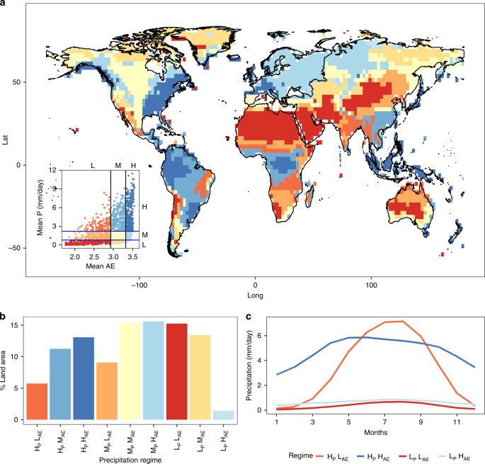
a Spatial distribution of precipitation regimes based on the percentile (Pri) thresholds concept using mean apportionment entropy (AE) and annual precipitation P during the 1971–2000 reference period. b Percentage of land occupied by each regime. c Precipitation climatology of the spatially aggregated monthly rainfall climatology for regimes HPLAE, HPHAE, LPHAE, LPLAE. These regimes are selected as they represent boundary case scenarios. H, M, and L represent high moderate and low values, respectively.
The spatial distribution of regimes across global land is found to be as follows: regime HPLAE and MPLAE can be found mostly in the Indian subcontinent, Northeast Asia, Northern Australia, and much of north-central and south-central Africa, covering land area of ~15%. These regions are influenced mostly by monsoons33. Regime HPMAE and HPHAE mostly occupy eastern North America, Northern South America, central Africa, Western Europe, and South Eastern Asia, occupying a combined land area of 24%. These regions are mostly moist forest areas. Regime MPMAE spans across most of central North America and is scattered in western parts of South America and Northern and central Asia, Southern part of Africa and Southern Australia amounting to ~15% of land area. Regime MPHAE occupies most of European Continent and further extends to western Russia occupying 16% of the total land area. Regime LPLAE occupies Northern Africa, the Middle East, and further extends to central Asia. In addition, central Australia, the interior western United States and central western South America are classified as belonging to LPLAE, occupying a land area of 15%. LPMAE is mostly confined to the Northern parts of North America and Siberia region occupying ~13% of land area. Finally, regime LPHAE is confined to a small region in the central Russian region.
Trends in annual changes of precipitation and evaporation
Precipitation and evaporation projections from Coupled Model Intercomparison Project Phase 5 (CMIP5) models are aggregated over these nine precipitation regimes. We evaluate linear trends over the 21st century (2005–2100) using Bayesian model averaging (BMA) (31–32, see “Methods”) applied to both annual means and seasonal variation in precipitation and evaporation for three future scenarios (representative concentration pathway (RCP) 2.6, 4.5, and 8.5).
The changes in BMA-weighted future annual precipitation and evaporation totals and seasonal variability for the RCP scenarios 2.6, 4.5, and 8.6 are shown in Fig. 2a, b, respectively (note that the horizontal axis scales are different for both panels in Fig. 2a, b). In Fig. 2a, the change in annual precipitation total (TOTP) indicates an increase in precipitation in all regimes, with the least increase in regime LPLAE, In addition, a proportional relationship was observed in terms of an increase in the precipitation magnitude with an increase in the emission forcing. In addition, in precipitation regimes LPHAE, MPHAE, and HPHAE that are characterized by a relatively consistent water supply, the TOTP exhibit a higher magnitude of precipitation increase compared with those regimes characterized by a moderate and high seasonal variability. Conversely, regions LPLAE, MPLAE, and HPLAE with inconsistent water supplies exhibit a lower magnitude of precipitation increase. The highest magnitude increase is evident in regime HPHAE, which is characterized by high volumes of consistent water supply in which RCP 8.5 exhibits an increase of 1.3 mm/year, followed by RCP 4.5 exhibiting 0.7 mm/year and RCP 2.6 exhibiting 0.25 mm/year. In addition, a larger uncertainty in the case of GCM model use is evident in precipitation regime HPHAE. Similar to TOTP, an increase in the annual evaporation total (TOTE) is observed in all regimes with the lowest increase observed in regime LPLAE. In addition, a direct proportional relationship is also evident here; the higher emission scenarios exhibit a higher magnitude of increased evaporation. As in the case of TOTP, TOTE in the precipitation regimes of LPHAE, MPHAE, and HPHAE that are characterized by relatively consistent water supply exhibit a higher magnitude of evaporation increase. The greatest change is evident in regime MPHAE, which is characterized by moderate precipitation but low seasonal variability. In this regime, RCP 8.5 exhibits an increase of 0.68 mm/year, followed by RCP 4.5 with an increase of 0.4 mm/year and RCP 2.6 with an increase of 0.19 mm/year. We observe that the changes in magnitude of TOTE are generally less uncertain than those in precipitation.
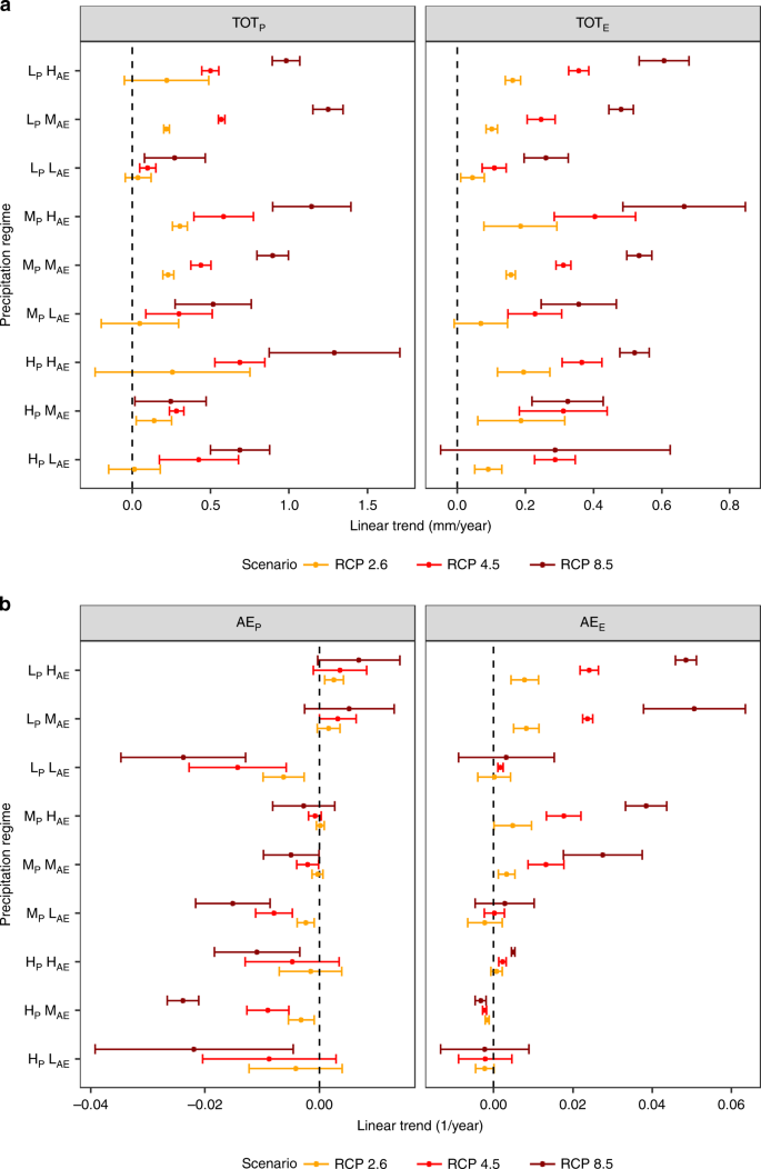
Theil-sen slopes of a total annual precipitation (TOTP) and total annual evaporation (TOTE) magnitudes, and b precipitation apportionment entropy (AEP) and evaporation apportionment entropy AEE. The error bars surrounding the point estimates represent the 95% confidence interval of the CMIP5 multimodel ensemble. H, M, and L represent high moderate and low values, respectively.
The decrease in AEP indicates an increase in the seasonal variability of precipitation in the regimes LPLAE, MPLAE, and HPLAE for all RCP scenarios as detailed in Fig. 2b. Although a negligible trend in RCP 2.6 is observed in case of regimes HPMAE, HPHAE, and MPMAE, a significant increase in variability was observed in the other scenarios for these three regimes. However, although a negligible positive trend is observed in regimes LPMAE and LPHAE for RCP 2.6, the other scenarios exhibit a decrease in variability. Regime MPHAE, which is characterized by moderate and consistent water supply exhibits a negligible change in all scenarios. Further, the changes in AEE are not as substantial as those in AEP. No significant trends are observed in AEE for regimes HPHAE, HPMAE, HPLAE, and MPLAE. In addition, decrease in variability of evaporation is evident in regime LPHAE, LPMAE, MPHAE, and MPMAE. The higher emission scenarios display greater change in magnitude for AEE. Unlike with precipitation variability, there is a pattern of decreased variability exhibited by AEE. These contrasting future projection changes in precipitation and evaporation may result in spatially variable monthly WA (i.e., P–E)6,31,34. To further assess the robustness of our results, we also computed the grid-wise trends as shown in Supplementary Figure 1 for RCP 8.5 scenario. Based on this spatially explicit analysis, we see that precipitation variability is increasing over a substantially greater region (~35.6% of the land surface) than it is decreasing (~4% of the land surface). In addition, the spatial analysis indicates that this increase in variability in more prominent in regions with high variability. Evaporation variability, conversely, is decreasing over a substantially greater region (~36% of the land surface) than it is increasing over (~6% of the land surface). Therefore, both these analyses suggested an overall trend toward increasing precipitation variability along with decreasing evaporation variability, reinforcing our main conclusions. As these metrics aggregate the monthly distributions of precipitation and evaporation at the annual scale obscuring seasonal behavior, it is worthwhile to additionally investigate, as described below, how these changes are reflected in the monthly distribution of available water (determined as the difference between precipitation and evaporation—See “Methods”).
Precipitation and evaporation role in available water change
We determine which seasonal components have contributed to altering the monthly distribution of WA (precipitation–evaporation) for each of these scenarios (See “Methods”). The BMA-weighted historical (1971–2000) monthly WA distribution and future projections (2070–2099) for each regime are shown in Fig. 3 for each of the scenarios. The projected future monthly distribution of WA for the wet seasons (8th–10th month) demonstrates that the wet season becomes wetter, a pattern that is increasingly evident in regimes LPHAE, MPHAE, and HPHAE with a consistent water supply albeit less evident in regimes LPLAE and MPLAE with an inconsistent water supply (regime HPLAE exhibits a minor increase in available water). So, while seasonally variable regimes becoming more variable in terms of precipitation, that is not the case for WA, perhaps owing to competing effects between evaporation and precipitation. The low precipitation of regime LPLAE exhibits the least noticeable change in monthly available water, unlike the high precipitation of regime HPLAE, wherein a more noticeable increase in available water is evident during the wet season. This pattern is also sensitive to the change in radiative forcing, with greater radiative forcing corresponding to greater changes. Therefore, in regions where water supply is constrained by low-precipitation amounts and a more uneven distribution (low AE), changes in precipitation and evaporation do not affect the available water as they are more water-limited in nature. In regions with a more even distribution, however, there is a greater effect. Overall, these results indicate that the changes in monthly WA distribution are dependent on both the particular regime and the radiative forcing.
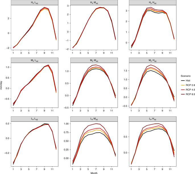
a BMA ensemble monthly projected (RCP 2.6, RCP 4.5, and RCP 8.5) of available water (2070–2099) and historical (1971–2000) scenarios. Where, H, M, and L abbreviate high moderate and low values, respectively. Whereas, apportionment entropy is abbreviated as AE and annual precipitation as P.
The corresponding changes in precipitation and evaporation (relative to the historical period) during the wet and dry seasons for three future emission scenarios (RCP 2.6, 4.5, 8.5) are presented in Fig. 4, illustrating the competition between water and energy balance at the seasonal scale. The role played by both wet and dry seasons in changing WA are examined in Fig. 4. In regions with high AE values (i.e., LPHAE, MPHAE, and HPHAE), higher increases in evaporation can be observed in comparison with the moderate and low AE regions, especially in the RCP 8.5 scenario. These changes are significant in the wet season but not the dry season. As noted earlier, higher emission scenarios show more pronounced evaporation increases. In the case of precipitation, regimes with high AE values in both dry and wet seasons display a pattern of increase similar to that in evaporation. But these changes are again only statistically significant in the wet season. Although greater changes in precipitation are evident in the dry season, the greater spread among models in that case hinders any confident conclusions.
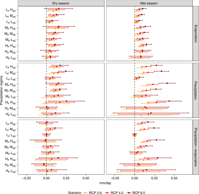
Relative changes in future precipitation and evaporation during the wet (three-month average with maximum precipitation in a year) and dry seasons (three-month average with minimum precipitation in a year) derived based on the CMIP5 scenario relative to the historical period (1971–2000). The error bars surrounding the point estimates represent the 95% confidence interval of the CMIP5 multimodel ensemble. H, M, and L abbreviate high moderate and low values, respectively. Whereas, apportionment entropy is abbreviated as AE and annual precipitation as P.
The increasing wet and dry season precipitation and evaporation provide an explanation for the changes in available water as defined by the difference between precipitation and evaporation (precipitation–evaporation). In regimes where the relative magnitude of the increase in evaporation is less than that in precipitation, a significant increase in WA is observed. Such is the case with high AE regions in wet season. This increase can thus be attributed to a larger increase in precipitation than in evaporation. In addition, regions with higher AE exhibit a greater increase in WA, which imply the potential for increased flood risk in regions such as Western Europe35, North America36, and South Eastern Asia that show less-seasonal variation16. In the case of the dry season, an increase in WA is found in RCP 8.5 scenarios for regimes LPMAE, MPMAE, and HPHAE but it is not statistically significant. The results in these cases are inconclusive owing to the large spread among models. This finding further highlights the interdependent role of evaporation and precipitation in changing seasonal WA. Previous studies based on spatially explicit analyses have shown that the dry seasons are becoming drier in some locations around the globe9. Our spatial analysis in case of RCP 8.5 scenario also indicates a decrease in P–E in Europe and northern part of North America (Supplementary Fig. 2) in agreement with Kumar et al.10,37.
Source: Resources - nature.com

