Data presentation
Managed concessions forest inventory data
The forest inventory dataset (hereafter CoFor dataset) corresponds to forest management inventories from 114 logging concessions (Fig. 2). Inventories followed standardized protocols22 and were conducted from the early 2000s to the early 2010s, at the exception of the Ngotto concession (1.4% of the data, sampled in 1993–1996) in the Central African Republic. Sampling designs were systematic and usually consisted of 20 to 25 m wide continuous and parallel transects, located 2 to 3 km apart, that were then aggregated into plots of 0.4 ha (8% of the cases) or 0.5 ha (91.7% of the cases). The remaining 0.3% of the plots ranged between 0.3 and 1 ha. Within each plot, information on tree diameter at breast height (DBH) and taxonomic identity were available for all trees with DBH ≥ 30 cm while smaller trees were either partially sampled or in some cases completely missing (see further). The quality of taxonomic information has been extensively reviewed elsewhere22. In total, the CoFor dataset contained 191,562 plots, covering a cumulated sampling area of 94,513 ha and representing 11.82 × 10⁶ tree measurements and 1,091 identified taxa.
Scientific forest inventory data
We used scientific forest inventory data to fine-tune and test the AGB computation scheme applied to forest management inventories and described in the next section. Scientific forest data were collated from plot networks and collaborators in Cameroon (IRD plot network23, CTFS Korup24 plot), Gabon (CTFS Rabi24 plot) and D.R. Congo25 (Fig. 2), and represented 233 1-ha plots. In each plot, the DBH of all trees with DBH ≥ 10 cm was measured and trees were identified following standard scientific protocols26. Forest structure in the scientific dataset covered most of the structural range found in CoFor, at the exception of forests characterized by both a small mean tree size and a low tree abundance (Supplementary Fig. 1), likely reflecting degraded forest states which can notably be found in Northern Congo (the so-called Marantaceae forests).
Estimation of plot and pixel aboveground biomass
Caveats of management inventories in forest concessions
Although the amount of information on central African forests structure and composition in the CoFor dataset is of unprecedented size and spatial representativeness, data collection protocols followed by forest companies do not conform to standard scientific protocols. This entailed additional computation steps and uncertainty sources when estimating forest sample plots aboveground biomass (AGB).
The first limitation of forest management inventories is that tree diameters are recorded as discrete (i.e. by 10 cm width bins), censored data rather than continuously. Tree diameter distributions were right-censored, meaning that all trees above a certain diameter threshold were pooled in a single ‘open class’. This diameter threshold varied across the 114 logging concessions (Fig. 3a) and mainly corresponded to 120 cm, 150 cm or 200 cm (8.9%, 47.8% and 11.5% of the sampling plots, respectively). Since tree AGB allometric models require continuous tree diameter values, it was necessary to establish a strategy to derive continuous DBH values from diameter classes (hereafter specific function 1).
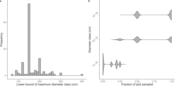
Caveats of forest management inventory data. (a) Frequency distribution of maximum diameter classes found across the 114 commercial inventories. For a given inventory, a maximum diameter class of e.g. 150 cm indicates that either 150–160 cm is the largest tree diameter class found in the field, or 150 cm is the opening threshold of the right-censored diameter distribution. (b) Frequency distributions of sampling rates (expressed as a plot fraction) for the three firsts diameter classes. For about half of the plots, trees in diameter class 10–20 cm were not sampled (i.e. plot fraction of 0), while trees in diameter class 30–40 cm were sampled on the entire plot area (i.e. plot fraction of 1). From diameter class 40–50 cm onward, trees were always sampled on the entire plot area.
Secondly, while a standard practice in scientific inventory protocols is to census all trees with DBH ≥ 10 cm, this census threshold can be higher in forest management inventory protocols and trees in the smallest diameter classes are not always sampled on the entire plot. In the CoFor dataset, for instance, the tree census threshold was 20 cm DBH in about half of the plots (i.e. 51.6%) and 10 cm DBH otherwise. Trees in the 20–30 and 30–40 cm DBH classes were sampled on the entire plot area in about half of the sampling plots (i.e. 42.7% and 58.4%, respectively) and partially sampled, most often on half of the plot area (Fig. 3b), in the remaining cases. When present, information on trees in the 10–20 cm DBH class was the least complete, as it typically corresponded to a sampling of 12.5% up to 33% of the plot area (Fig. 3b). Since forest AGB is commonly reported for all trees ≥ 10 cm DBH in the scientific literature, we developed procedures to correct for the partial inventory (hereafter specific function 2) or complete absence (hereafter specific function 3) of small trees in forest management inventories.
Computation scheme
We built a complete computation scheme to derive standardized estimates of plot AGB and associated errors from the CoFor dataset using a Monte Carlo approach (see Fig. 4 for a general overview). The general workflow can be decomposed into three main steps. First, forest management inventory data were transformed so as to mimic the format of scientific inventory data, which implied to (i) simulate the abundance of small trees in partially-sampled diameter classes (specific function 2) and (ii) assign continuous tree diameters from discrete diameter classes (specific function 1). Second, we used the BIOMASS R package27 for computing standardized plot AGB from inventory data using the pantropical AGB allometric model28 and for error propagation. Package’s build-in functions were used to retrieve tree wood density from the Global Wood density database29 and tree height using Feldpausch’s height-diameter allometric model30 parametrized for the central African region. An estimate of plots AGB was then obtained from trees AGB and either corresponded to the AGB above 10 cm DBH (when trees in the 10–20 cm DBH class were partially sampled in the plot) or above 20 cm DBH (when trees in the 10–20 cm DBH class were not sampled in the plot). In this last case, a third step consisted in applying a correction to plots AGB estimations (i.e. specific function 3) to predict plots AGB above the standard 10 cm DBH threshold.
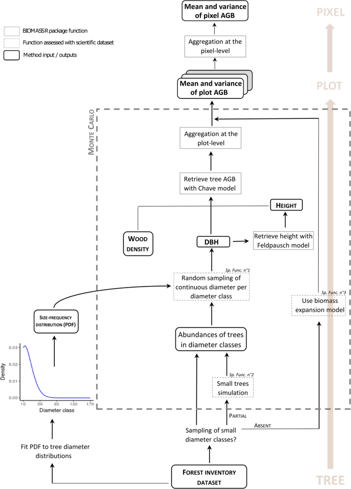
Workflow of aboveground biomass (AGB) computation scheme from forest management inventory data to plot and pixel estimations. The three specific functions (noted Sp. Func.) developed for this study are framed with dashed lines (see sections below for details).
For each plot, we generated 1000 AGB estimates using a Monte Carlo procedure. For each Monte Carlo simulation, errors associated to each computational step are calculated and propagated throughout the computation chain. This approach has been described elsewhere, notably in the BIOMASS R package27, and is now used as a standard for generating calibration AGB data for satellite missions31. The procedure outputs a vector of AGB estimates for each plot (of length 1000 here) from which we extracted the mean and the variance. The mean of AGB estimates within plots was used as the plot AGB value, while the variance and the coefficient of variation (CV) were used to compute estimation uncertainty. Besides classical error sources handled by the BIOMASS R package, an important aspect of our preliminary analyses was to quantify the errors associated to the three specific functions introduced below to deal with the peculiarities of forest management inventory data and for which we used scientific forest inventory as test data (see Technical Validation section).
Once computed, plot-level AGB estimates were aggregated into 1-km pixels using the weighted mean function of the SDMTools R package32, with plots area as the set of weights. The resulting 59,857 pixels map represented in Fig. 1 provides the first overview of large-scale spatial variation in African moist forests AGB derived from field data. Anticipating users’ needs for pixel-level AGB uncertainty assessments, we also computed (i) the weighted mean of within-pixel plots AGB variance (corresponding to intra-plot variance) and (ii) the weighted variance of within-pixel plots mean AGB (corresponding to inter-plot variance). Summing the intra- and inter-plot variances yields pixel-level total variance, which we expressed as a coefficient of variation (in %) to report on the total AGB uncertainty at the pixel scale. Intra- and inter-plot variances were also separately expressed as coefficients of variation (in %), and are hereafter referred to as estimation uncertainty and sampling uncertainty, respectively.
Specific function 1: assignment of tree diameters from diameter classes
Assigning continuous tree diameter values from a discrete, censored distribution requires positing (i) a probability distribution function (PDF) for continuous tree diameters within each diameter class and (ii) the maximum diameter (Dmax) a tree may reach in the open diameter class (e.g. 150–Dmax cm). In preliminary testing, we used the forest management inventory dataset to fit three probability distribution functions, namely an exponential distribution, a two-parameter Weibull distribution and a two-parameter Gamma distribution, each time considering a set of realistic Dmax values (i.e. from 300 to 500 cm by 50 cm steps). Distribution functions were fitted either by genus or considering all genera simultaneously. A weighted AIC was used to select the distribution that best fitted the data. We then assessed how well these different strategies (i.e. genus-specific or generic PDFs, distribution function type) allowed estimating actual plot AGB using the set of scientific forest plots. Continuous tree diameters in the scientific inventory dataset were discretized, and we used the fitted PDFs to generate continuous tree diameter by inverse transform sampling33. We then compared plot AGB estimates derived from degraded and original data. Based on 1000 iterations of the Monte Carlo scheme on the scientific dataset, we found that Dmax value had little influence on the results and that using genus-specific PDFs rather than a single generic PDF did not significantly reduce AGB estimation errors. In the final AGB computation scheme (Fig. 4), we thus arbitrarily set Dmax to 400 cm and selected the best generic PDF, i.e. the 2-parameter Weibull distribution function, with a scale parameter λ = 8.593 and a shape parameter k = 0.737.
Specific function 2: simulation of small tree data in partially-sampled diameter classes
Forest management inventory data often contain a partial sampling of trees in the smallest diameter classes, i.e. trees in diameter class i are sampled in a spatial fraction p of the plots, with i and p varying across logging companies (Fig. 3b). To compute plot AGB for all trees ≥ 10 cm DBH, it was necessary to account for trees that were not sampled. Here, we developed a two-step procedure to simulate missing tree data: at each iteration of the plot AGB Monte Carlo computation, we (i) expanded the tree count r observed in a given diameter class and plot from the spatial fraction p to the entire plot by randomly generating a value from a negative binomial distribution X ~ NegBin(r, p), and (ii) assigned species labels to simulated trees at the pro-rata of species abundance observed in the p fraction of the plot.
Specific function 3: biomass correction model for trees in diameter class 10–20 cm
To predict the total biomass of plots where trees in diameter class 10–20 cm were not sampled, we developed a biomass correction model using c. 90,000 forest management plots where trees in the 10–20 cm diameter class were partially sampled. In preliminary testing, we first computed AGB of trees in the 10–20 cm diameter class (AGB10–20) and above 20 cm (AGB≥20) for each plot, as the average of 1000 AGB simulations while propagating classical errors (on wood density, height-diameter and AGB allometric models) as well as errors on the simulation of small trees and diameter assignment functions inherent to our AGB Monte Carlo computation scheme. Across forest management plots, AGB10-20 represented on average 10.1 ± 8.6% of AGB≥20, close to what was found on the scientific dataset (11.3 ± 7.9%). Then, we tested several simple linear models to predict AGB10-20, using the set of 90,000 plots as calibration data and scientific plots as validation data. Using AGB≥20 as sole model predictor led to a poor calibration fit (R²calib. of 0.04, Fig. S5a) and predictive power (R²valid. of 0.02 on scientific plots). In order to improve the AGB10-20 model, we thus computed two additional metrics, S and I, describing the shape of plots cumulated biomass distribution function (Fig. 5b). S and I correspond respectively to the slope and the intercept of a simple linear model calibrated on plots’ cumulated biomass by 10 cm classes, from 20 cm up to 70 cm. The distribution of S and I on commercial data was consistent with that found on scientific data (Fig. 5c). We found that including S and I in the AGB10-20 model led to a significant improvement (although modest) of its calibration fit (R²calib. of 0.18) and predictive power (R2valid. of 0.29 on scientific plots). In the final AGB computation scheme (Fig. 4), we therefore retained this model to predict AGB10-20:
$$AG{B}_{10-20}=a+bast AG{B}_{ge 20}+cast S+dast I+varepsilon $$
where a, b, c and d are model coefficients and ε is the error term, assumed to follow a normal distribution N ~ (0, ε²), with ε the residual standard error of the model.
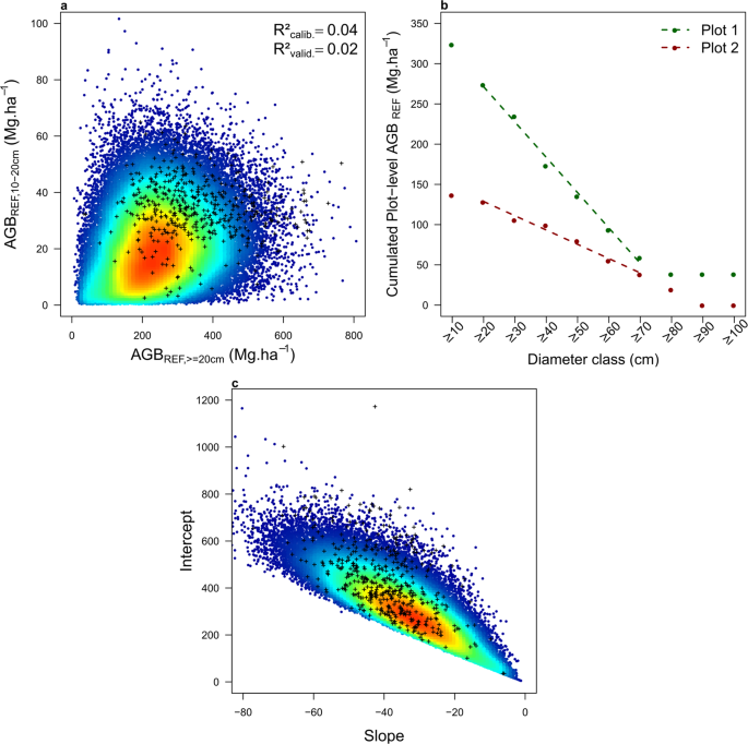
Biomass correction model for trees in diameter class 10–20 cm. (a) Heat plot showing the relationship between tree AGB in the 10–20 cm diameter class vs AGB of trees ≥ 20 cm diameter in commercial inventories, overlaid by the scientific dataset (small black crosses). (b) Shape of the cumulated AGB distribution across 10 cm wide diameter bins for two illustrative plots, with dashed lines representing the fit of the linear models of slope S and intercept I. (c) Heat plot showing the relationship between S and I in commercial inventories, overlaid by the scientific dataset (small black crosses).
Source: Ecology - nature.com
