A minimal model for microbial biodiversity can reproduce experimentally observed ecological patterns

All synthetic data was generated using the Microbial Consumer Resource Model previously described^9,10 and summarized below. We found the fixed points of the dynamics for each community using the Python package Community Simulator¹⁰: https://github.com/Emergent-Behaviors-in-Biology/community-simulator. Principal Coordinate Analysis was performed on the simulated HMP data using the Python package scikit-bio http://scikit-bio.org/. The pairwise distance matrix was generated using standard scipy commands with the Jensen-Shannon distance metric. Dissimilarity-overlap analysis was performed on the simulation data following the procedure described in Ref. ³³. All simulation data and analysis scripts are available at https://github.com/Emergent-Behaviors-in-Biology/microbiome-patterns.

MiCRM dynamical equations

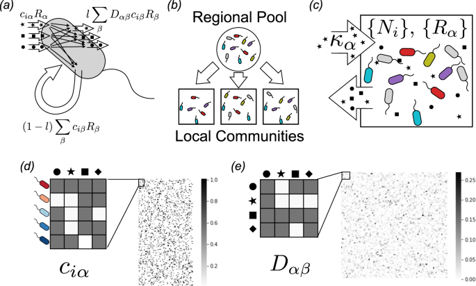
We consider the dynamics of the population densities N_i of S microbial species and the abundances R_α of M resource types in a well-mixed system, governed by the following set of ordinary differential equations:

For this study, the conversion factors g_i from energy uptake to population growth were all set to 1, as were the resource qualities w_α and the resource dilution rate ({tau }_{R}^{-1}). The leakage fractions l_α govern how much of each consumed resource is released into the environment as metabolic byproducts, and was set to 0.8 for all α. See Table 1 for list of all parameters and units.

Random sampling of consumer preference matrix and metabolic matrix

As noted in the Introduction, modeling highly diverse communities such as microbiomes requires a large number of free parameters. For example, the simulations with 5,000 species performed here required choosing over a million parameter values. In order to explore the typical phenomena produced by our model, we sampled the parameters randomly. Under the sampling scheme described in this section, the model is fully defined by a choice of just twelve parameters, listed in Table 2.

We choose consumer preferences c_iα as follows. We assume that each specialist family has a preference for one resource class A (where A = 1…F) with 0 ≤ F ≤ T, and we denote the consumer coefficients for this family by ({c}_{ialpha }^{A}). We also consider generalists that have no preferences, with consumer coefficients ({c}_{ialpha }^{{rm{gen}}}). The ({c}_{ialpha }^{A}) can be drawn from one of three probability distributions : (i) a Normal/Gaussian distribution, (ii) a Gamma distribution (which ensure positivity of the coefficients), and (iii) a Bernoulli distribution with binary preference levels.

The key parameters for constructing all three distributions are the mean μ_c and the variance ({sigma }_{c}^{2}) of the sum ∑_αc_iα over a row of the matrix.

In the current study, we focus on binary preference levels (option iii). In this model, there are two possible values for each c_iα: a low level (frac{{c}_{0}}{M}) and a high level (frac{{c}_{0}}{M}+{c}_{1}). For a given choice of μ_c, the parameters c₀ and c₁ together determine the variance ({sigma }_{c}^{2}). The elements of ({c}_{ialpha }^{A}) are given by

where X_iα is a binary random variable that equals 1 with probability

for the specialist families, and

for the generalists.

We choose the metabolic matrix D_αβ according to the three-tiered secretion model depicted in Fig. 4. The first tier is a preferred class of ‘waste’ products, such as carboyxlic acids for fermentative and respiro-fermentative bacteria, with M_w members. The second tier contains byproducts of the same class as the input resource (when the input resource is not in the preferred byproduct class). For example, this could be attributed to the partial oxidation of sugars into sugar alcohols, or the antiporter behavior of various amino acid transporters. The third tier includes everything else. We encode this structure in D_αβ by sampling each column β of the matrix from a Dirichlet distribution with concentration parameters d_αβ that depend on the byproduct tier, so that on average a fraction f_w of the secreted flux goes to the first tier, while a fraction f_s goes to the second tier, and the rest goes to the third. The Dirichlet distribution has the property that each sampled vector sums to 1, making it a natural way of randomly allocating a fixed total quantity (such as the total secretion flux from a given input). To write the expressions for these parameters explicitly, we let A(α) represent the class containing resource α, and let w represent the ‘waste’ class. We also introduce a parameter s that controls the sparsity of the reaction network, ranging from a dense network with all-to-all connection when s → 0, to maximal sparsity with each input resource having just one randomly chosen output resource as s → 1. With this notation, we have

The final two lines handle the case when the ‘waste’ type is being consumed. In this case, the fraction allocated to the waste type is the sum of the fractions allocated to ‘same’ and ‘waste’.

Solving for uninvadable equilibrium

We computed the uninvadable equilibrium state of Equation (2) using a novel algorithm inspired by expectation-maximization methods in machine learning. The algorithm is described in detail in Ref. ¹⁰, and implemented computationally in the Community Simulator package.

The raw results of the computation have nonzero abundances for all species, due to technical limits on numerical precision in the solver. In all simulations, the abundance distribution was clearly bimodal, with well-separated peaks on a log scale for the surviving vs. extinct species. For purposes of determining species richness, we set the abundance of all species in the “extinct” group to zero. Histograms of the raw results are plotted in the accompanying Jupyter notebook, where the choice of threshold for removing extinct species can be directly verified.

The large simulations with 300 resources and 5,000 species pushed the limits of our implementation of the algorithm, and occasionally failed to converge. Before performing further analysis, we directly verified that a true solution had been found by calculating the per-capita growth rate (d {rm{ln}}, {N}_{i})/dt for all surviving species. A histogram of the maximum value of (| d {rm{ln}}, {N}_{i}/dt| ) for each community (on a log scale) shows that most simulations are around 10⁻⁷, with the upper tail reaching to around 10⁻⁵. In the least stable simulation, with S = 4, 900 and two externally supplied resources, the failed runs form a second cluster around (| d {rm{ln}}, {N}_{i}/dt| =1{0}^{-3}). To eliminate such runs, we set a threshold for all simulations discarding samples with (| d {rm{ln}}, {N}_{i}/dt| ge 1{0}^{-5}). For the least stable scenario, 29 of the 900 samples exceeded the threshold, and all others had between 0 and 11.

Synthetic data for global biodiversity patterns

Synthetic data for Figs. 2 and 3 was generated using a regional species pool of size S_tot = 180 and M = 90 potential resources. The elements of the 180 × 90 consumer preference matrix c_iα were sampled from a binary distribution as described above, with c₀ = 0, c₁ = 1 and μ_c = 10, using only one resource class (T = 1) and one consumer family (F = 1). The 90 × 90 metabolic matrix D_αβ was sampled from a Dirichlet distribution as described above, with s = 0.05. The m_i were sampled from a Gaussian distribution with mean 1 and standard deviation 0.01. A random number from a uniform distribution between − 0.5 and 9.5 was added to all the m_i’s from each sample.

The rest of the parameters differed among the three scenarios we simulated, and were chosen as follows:

• Simple environment (same as “selection-limited” in Fig. 3): Each sample was stochastically colonized with S = 150 out of the 180 possible species, and supplied with a single external resource, with κ₁ = 200 and κ_α = 0 for all α ≠ 1.

• Complex environment: Each sample was stochastically colonized with S = 150 out of the 180 possible species, and supplied with all external resources, with κ_α = 200/M = 2.2 for all α.

• Dispersal limited: Each sample was stochastically colonized with a randomly chosen number of species, uniformly distributed between S = 1 and S = S_tot = 180, and supplied with a single external resource, with κ₁ = 200 and κ_α = 0 for all α ≠ 1.

Synthetic data for human microbiome patterns

To generate synthetic data for Figs. 6–9, we assumed a regional species pool of size S_tot = 5000, with M = 300 possible resource types. Resources were grouped into T = 6 classes of 50 resource types each, labeled A through F. Microbial species were grouped into 6 specialist ‘‘families” of 800 species, with each family specializing in one resource class as described above. The remaining 200 species were designated as generalists, with no bias towards any one resource class. The consumption parameters were set to c₀ = 0, c₁ = 1 and μ_c = 10 as for the previous set of simulations. The metabolic matrix sparsity was set to s = 0.3, to reflect the actual sparsity of the E. Coli metabolic network³⁸, and the secretions were allocated with f_s = f_w = 0.45. The m_i were sampled from a Gaussian distribution with mean 1 and standard deviation 0.01. Each community was supplied with the same total incoming energy flux κ = ∑_ακ_α = 1, 000. For each scenario, we simulated 900 independent communities, evenly partitioned among three “body sites” with different environmental characteristics.

The rest of the parameters were varied to construct eight different scenarios. For S = 2, 500 (strong dispersal limitation) and S = 4, 900 (weak dispersal limitation), we made the following four combinations of species properties and environmental conditions:

• Metabolically distinct simple environments: In each of the three simulated body sites, one resource was chosen from each of two resource classes (A + B, C + D, and E + F). The relative flux levels for these two resources were chosen for each of the 300 communities in the site by randomly sampling a number a from a uniform distribution over the interval [0, 1], and then letting (1 − a)κ be the flux of the first resource, with aκ from the second. Taxonomic structure was incorporated by setting a high strength of specialization q = 0.9.

• Metabolically distinct complex environments: In each of the three simulated body sites, all resources were supplied from two resource classes (A + B, C + D, and E + F), with flux levels from all other classes still set to zero. The relative flux levels for 100 resource types in each site were randomly sampled for each community, by independently sampling 100 numbers ({widetilde{kappa }}_{alpha }) from a uniform distribution over the interval [0, 1], and then setting ({kappa }_{alpha }=kappa frac{{widetilde{kappa }}_{alpha }}{{sum }_{beta }{widetilde{kappa }}_{beta }}). Taxonomic structure was incorporated by setting a high strength of specialization q = 0.9.

• No taxonomic structure: Same as “metabolically distinct simple environments” above, except that taxonomic structure was removed by setting q = 0.

• Metabolically overlapping complex environments: Same as “metabolically distinct complex environments” except that the 300 resources were randomly partitioned into three sets of 100, and each body site was supplied with resources from a different set.

Synthetic data for marine microbiome patterns

The abundance distributions in Fig. 5 were generated directly from the “Simple environments” and “No taxonomic structure” simulations described above for the human microbiome patterns.

The tests of modular community assembly in Fig. 10 were performed using the same setup as “Simple environments” in the human microbiome simulations, but with just two “body sites” (A + B and C + D), and three values of a (0, 1 and 0.5). The unstructured metabolism control was performed by setting T = F = 1, assigning all 300 resources to the same resource class before sampling the metabolic and consumer preference matrices.

Relative abundance distributions and fisher log series

To create Fig. 5, we first downloaded the 16S OTU table from the Tara Oceans companion website (http://ocean-microbiome.embl.de/companion.html)²⁰. We performed 300 independent rarefactions to a constant read depth of 10,000. For each possible number of reads, from 1 through the maximum observed, we plotted the number of species assigned that number of reads (“population size”), averaged over all rarefactions.

In many ecological settings, it has been observed that the number s(n) of species with n individuals in a sample of N total individuals closely follows the Fisher log series^25,26:

where the parameters x and α are determined from N and the total number of observed species S through the following equations:

In the first panel of Fig. 5 we plot Eq. (8) using N = 10, 000 (the read depth we manually imposed for the rarefaction) and S equal to the number of OTU’s with more than 5 reads assigned to them in the original dataset.

For the simulation data in Fig. 5, we had the further advantage of having access to multiple independent trials under statistically similar conditions. Instead of averaging over multiple rarefactions generated from the same underlying dataset, we averaged over single samples of N = 1, 000 individuals taken from each of the 900 parallel communities. We plotted the Fisher log series with N = 1, 000 and S equal to the number of species with nonzero abundance.

We also plotted the distributions obtained when the underlying relative proportions of S species are generated by a simple null model, in which the invasion fitness (low-density growth rate) of each species is sampled from a Gaussian distribution. Species with negative values go extinct, and those with positive values end up with population sizes proportional to the invasion fitness. The resulting relative abundances of species in an infinitely large community follow a truncated Gaussian distribution. This distribution is determined by a single parameter, up to an overall scale that is irrelevant for the purposes of the current analysis. The parameter is inferred from the simulation results by matching the fraction of species initially present in the community that survive to equilibrium. In the figure, the green curves come from first sampling S underlying species abundances from this distribution, then sampling N = 1, 000 individuals from the resulting population, and averaging the results over 10,000 independent iterations.

Computation of overlap and dissimilarity

Here we summarize the definitions of the dissimilarity (D({{N}_{i}^{mu }},{{N}_{j}^{nu }})) and overlap (O({{N}_{i}^{mu }},{{N}_{j}^{nu }})) between two sets of population size measurements, as given in Ref. ³³. Here, μ = 1, 2, …C is an index labeling the sample from which the measurement was taken (as is ν). In order to define these two quantities, we must first introduce some notation concerning the shared species. We let S^† represent the set of species that are present in both communities, and denote the total number of species in this set by S^†. We also define two types of normalized abundances:

where the second quantity is normalized only by the set of species that is shared with the other community in the pair. We also define the average composition over the shared species:

Using these definitions, we can finally write

The first equation is simply the square root of the Jensen-Shannon divergence between the relative abundances of the overlapping species, and the second measures the relative abundance of the species in the overlapping set, averaged over the two communities.

Computation of effective Lotka-Volterra parameters

The distinction between “host-specific” vs. “universal” population dynamics is most clearly defined in terms of a closed set of equations for the dynamics of the population sizes, with environmental factors treated implicitly³³. We can transform the MiCRM into a model of this form by examining the regime where the resource dynamics are “fast” compared to the timescale for changes in population sizes. We can then simplify the form of the resulting model by performing a Taylor expansion of the growth rate around the equilibrium population sizes ({bar{N}}_{i}), resulting in generalized Lotka-Volterra equations parameterized by a set of carrying capacities and interaction coefficients.

We start by writing the full dynamical equation (2) in a more compact form:

with

We now invoke the “fast resource equilibration” assumption to set dR_α/dt = 0, and solve for the resource concentrations ({bar{R}}_{alpha }) as functions of the set of population sizes {N_j}. Inserting this result back into the equations for the dynamics of N_i, we have:

To obtain the local Lotka-Volterra coefficients, we perform a Taylor expansion of the term in brackets around ({N}_{j}={bar{N}}_{j}), up to first order in the distance from equilibrium:

where

We can compute the derivatives of (bar{R}) through implicit differentiation to obtain

with

Thus we find

and conclude

where

Since all the parameters and equilibrium abundances are known in the simulations, this set of equations allows us to compute for each community μ (μ = 1, 2…300) the bare growth rates ({r}_{i}^{mu }), the interactions ({alpha }_{ij}^{mu }) and the carrying capacities ({K}_{i}^{mu }). The scatter plot in the bottom right panel of Fig. 9 shows the normalized RMS variability in the carrying capacities for each pair of samples μ and ν, computed as:

where S^† is the number of surviving species shared between the two communities, and S^† is the set of indices of the shared species.

Source: Ecology - nature.com