An analysis of optimal fertigation implications in different soils on reducing environmental impacts of agricultural nitrate leaching

Micro-irrigation system

This research carried out based on experiments and measurements conducted in 2016 on a corn field with surface drip irrigation system in the location of Urmia University, Iran (detailed given by Azad et al.²²). In the mentioned study, the HYDRUS-2D model and the proposed optimization algorithm were calibrated using field data collected by the authors. N plant uptake and leaching were simulated in this study in three different scenarios of N fertilizer applications for corn in a system with surface drip- irrigation. All simulations were carried out for three different soil types of silty clay (C), loam (L), and sandy loam (SL). The common corn variety grown in the northwest of Iran-Urmia plain was considered. The growth period of this variety of corn is 16 weeks, and a typical planting layout is shown in Fig. 1a.

Figure 1

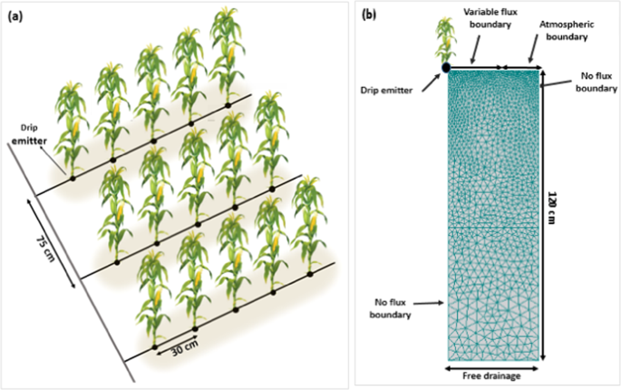
Layout of the driplines and plants (a) and the conceptual geometry and boundary conditions in the HYDRUS-2D simulations (b).

Full size image

Irrigation was considered twice a week in the silty clay and loamy soils and three times a week in the sandy loam soil (Fig. 2) at the irrigation flow rate of 4 L h⁻¹. Irrigation intervals choosing was based on the maximum allowed irrigation intervals according to water holding capacity of the soil and preventing water deep percolation²³. Potential evapotranspiration of corn was calculated to determine the water irrigation depth and the duration of irrigation in each irrigation event. Total amount of irrigation water was constant in all soils. Potential crop evapotranspiration (ET_p) was calculated using the reference crop evapotranspiration (ET_o) based on the FAO Penman-Monteith equation and the dual crop coefficient approach²⁴. Meteorological data required to calculate ET_o were obtained from the meteorological station at the study area. The corn N requirement, based on local recommendations, was 113.5 kg ha⁻¹ N. Therefore, 334 kg ha⁻¹ of ammonium nitrate fertilizer was considered for the growing season.

Figure 2

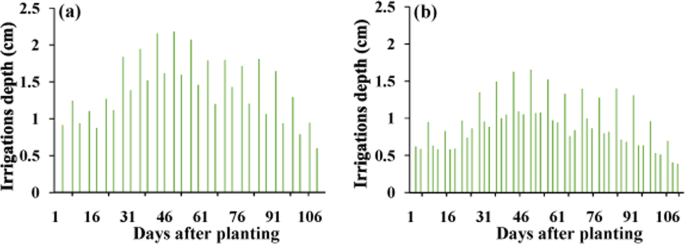
Irrigation depths for (a) silty clay and loamy soil (2 irrigation events per week) and (b) sandy loam soil (3 irrigation events per week) scenarios.

Full size image

Simulation model

The HYDRUS (2D/3D) model^12,25 was used in this research to simulate water flow, solute movement, plant root growth, and root water and nutrient uptake in a two-dimensional soil profile. This program numerically solves the Richards²⁶ equation for variably-saturated water movement and a convection-dispersion equation for solute transport in soil using the Galerkin finite element method.

A 2D-vertical plane (two-dimensional transport domain) with a width of 37.5 cm and a depth of 120 cm was defined in the HYDRUS-2D model (Fig. 1b). A strip wetting pattern along the driplines was represented in the model using a time-variable flux boundary condition on the left side of the soil surface, through which water and solutes entered the soil profile during irrigation/fertigation events. The third-type Cauchy boundary condition was used in this area to allow the entry of solutes at the soil surface during fertigation events. The atmospheric boundary condition (with evaporation) was specified on the rest of the soil surface.

Root growth and root densities in lateral and vertical directions were simulated using a recently developed computational module of HYDRUS-2D^22,27,28. In this module, the dynamic rooting depth can be calculated as follows²⁹:

where ({L}_{R}(t)) is the root length at any time (depth: (Z(t)) and radius: (X(t)), L_m is the maximum root length (maximum depth: Z_m and maximum radius: X_m) and t is days after planting. In this equation, f_r(t) is a dimensionless root growth function. This function is calculated using the classical Verhulst-Pearl logistic growth equation:

where L₀ is the initial value of the rooting depth (recommended value=1 cm) and r is the growth rate (T⁻¹). The growth rate, r, is calculated either from given data of the rooting depth at a specific time or from the assumption that 50% of the rooting depth is reached after 50% of the growing season. The second approach was used in this study. When a variable rooting depth is considered, the spatial distribution of roots must be described using either the Vrugt^30,31 or Hoffman and van Genuchten³² functions. The Vrugt’s root distribution function was used to simulate both the vertical and horizontal growth of the roots.

The maximum depth and radius of the corn roots were considered to be 60 and 35 cm^6,33, respectively. Similarly, as in Wang et al.³³, the parameters defining the maximum root water uptake intensity in vertical and horizontal directions (z^* and x^*) were selected to be 10 and 0 cm, respectively, and the shape coefficients p_x and p_z were set to 1.0. The reduction of root water uptake due to the water stress was described using the macroscopic approach of Feddes et al.³⁴ with specific corn coefficients from the HYDRUS-2D database³⁵.

HYDRUS-2D uses the van Genuchten-Mualem functions³⁶ to describe soil hydraulic properties, i.e., retention curves and hydraulic conductivity functions. The parameters for these relationships (i.e., the residual water content θ_r, the saturated water content θ_s, the van Genuchten shape parameters [α, n, and l], and the saturated hydraulic conductivity K_s) were taken for loam and sandy loam from Carsel and Parish³⁷ and for silty clay from the Rosetta database³⁸, similarly as done by Gärdenäs et al.¹³. The soil hydraulic parameter values are listed in Table 1.

The convection-dispersion equation and the first-order decay chain were used to simulate the transport and transformations of N species, respectively. These equations and their parameters are described in Šimůnek et al.³⁹. Since ammonium nitrate was considered as a fertilizer, ammonium adsorption to the soil particles and nitrification (NH₄⁺ transformation into NO₂⁻ and then further into NO₃⁻) were considered as the main reaction processes. The distribution coefficient (K_d) for ammonium sorption and the first-order rate constants for nitrification of ammonium to nitrate in the liquid and solid phases (µ′_w and µ′_s, respectively) were specified using parameters reported in the literature^{13,14,16,33,40,41}: 3.5 cm³ gr⁻¹, 0.2 day⁻¹, and 0.2 day⁻¹ for K_d, µ′_w, and µ′_s, respectively. The longitudinal dispersivity (ε_L) and the transverse dispersivity (ε_T) were set to be one-tenth of the soil depth and one-tenth of ε_L, respectively¹⁶. The initial concentrations of ammonium and nitrate were set to a uniform zero concentration similar to the research of Gardenas et al.¹³. Similarly as in many other studies^{14,15,16,41,42} mineralization and immobilization were neglected. Furthermore, in drip irrigation, the process of denitrification can be neglected due to unsaturated and aerobic conditions in the soil⁴¹. Similar to the present study, in the research of Gardenas et al.¹³ denitrification losses were ignored in silty-clay, loam and sandy loam soils in the micro-irrigation system. Finally, similar to the study of Ramos et al.¹⁶, unlimited passive nutrient uptake⁴³ was considered for N species. The N balance components, including accumulation and leaching, were evaluated for the root zone 65 cm deep.

Fertigation scenarios and optimization of fertigation scheduling

In the first step, water flow, water uptake by plants, plant growth, solutes transport, nitrate leaching, and N uptake by plants were investigated by considering two different fertigation scenarios with fixed application frequencies during the growing season. In the first fertigation scenario, fertilizer applications were divided into three splits, which are used by local farmers. In this scenario, 50, 25, and 25% of the total N fertilizer was applied at the beginning of the growing season, at the knee stage, and at the tasselling stage, respectively. In the second fertigation scenario, the fertilizer was applied weekly throughout the entire growing season. In both cases, the fertilizer was applied at the end of the irrigation event (before providing the opportunity to wash the pipes and emitters after the fertilizer application). The duration of the fertilizer application in each fertigation event was based on the minimum allowed period of the application to meet the criteria of EC < 3 dS m⁻¹ of the irrigation water⁴⁴. The minimum application time was considered to be 5 minutes.

In the second step, the design and management parameters of irrigation and fertigation (including irrigation flow rate, duration and start time of fertigation and also, fertilizer amounts in each fertigation event) were optimized for three soil textural types. The objective of this optimization was to increase N uptake sufficiency and to decrease environmental contamination due to nitrate leaching. It should be noted that in addition to nitrate leaching from the soil profile throughout the growing season, nitrate accumulated in the soil profile at the end of the growing season will likely also leach from the soil profile and be transported to groundwater aquifers due to autumn and winter precipitation after crop harvesting. In fact, both nitrate leaching during the growing season and its accumulation at the end of the growing season in the soil profile should be avoided when optimizing design and management parameters of fertigation.

Optimization was done in two stages. First, the irrigation flow rate (Q), the start time of the fertilizer application (T_start), and the duration of fertigation (T_fer) were optimized for each soil type to minimize nitrate leaching. The objective function was as follows:

where (,OF1) is the objective function of the first stage of optimization, ({D}_{wp}) is deep water percolation and (N{O}_{3}^{-}_L) is leached nitrate. These components are dimensionless as a fraction of the input value of water or nitrate. The optimization was carried out for a duration of one week with two or three irrigation events (depending on the soil texture) while fertigation was applied in the first irrigation event of the week. This approach allowed us to consider the effects of subsequent irrigation events (one or two) without fertigation on nitrate leaching.

Second, after determining the best combination of decision variables (i.e., Q, T_start, and T_fer), the fertilizer amounts were optimized for each fertigation event of the growing season based on the plant’s N demand at different stages of the plant growth. Besides supplying plant’s N requirements, nitrate leaching during the growing season and nitrate accumulation in the soil profile at the end of the growing season were minimized. The objective function was as follows:

where (,OF2) is objective function of the second stage of optimization, ({S}_{diff}) is cumulative difference between the plant demand and uptaken N, (N{O}_{3}^{-}_Losses) is total leached and accumulated nitrate in the soil. The minimum allowed duration of the fertilizer application for optimized irrigation rates was set to prevent exceeding maximum irrigation water salinity (EC_iw < 3 dS m⁻¹). Additional explanations about the objective functions, decision variables, and constraints of the optimization model during the two optimization stages are given in Azad et al.²². The Particle Swarm Optimization (PSO) method^45,46 was employed in the optimization process. Optimization was run in MATLAB linked with the HYDRUS-2D model.

Source: Ecology - nature.com