An interspecific variation in rhizosphere effects on soil anti-erodibility

Study area and key species

This study was performed in the area surrounding Guiyang city, Guizhou Province, China (26º17′-26º22′ N, 106°07′-107°17′ E; 506–1762 m), which is characterized by karst formations and seminatural forests. We selected 42 plant species with key roles in structuring the karst evergreen broadleaf forests and seven forest sites (Fig. 6) where these species occur, in accordance with Huang et al.²⁰. These species belong to 21 families (Supplementary Material S3) and include both evergreen (22) and deciduous (20) species. The species are dominant or edificator species and are usually rooted within fissures on the karst substrate (Fig. 6B, Supplementary Material S4). The root systems of these species filled nearly all the spaces in the soil fissures (Fig. 6C), thereby playing a major role in all soil processes.

Figure 6

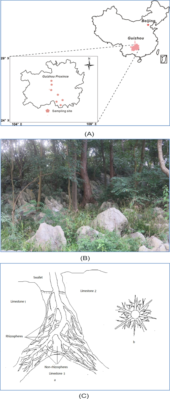
Sampling sites. (A) Locations of sampling sites; (B) plants growing in fissures; (C) the root system of a plant growing in a fissure. In (C), a and b represent the longitudinal and cross-sectional sections of root systems, respectively.

Full size image

Soil sampling

We identified seven forest sites (Fig. 6) in which the target species were known to occur according to previous studies²⁰. Afterward, 20 m × 20 m plots with similar habitats were established in each site. We successively searched for three individual plants of each species in each plot according to the typical conditions of the adult plants, ensuring similar ages (15–20 years old; at such an age, plants vigorously grow with a high secretion of root exudates), canopy coverage, tree height, and diameter at breast height. If three similar individuals of one species were not located within a plot, we continually searched in subsequent plots. The final number of plots within the 7 forest sites was 129. After the identification of three individuals per species, the soil in the fissure was removed in successive layers. After finding living fibrous roots, we used the stripping method to remove the external (thickness > 1 cm) soil around the roots and collected 500 g of inner soil (0–1 cm thickness) per tree¹³. The sampling diameter of the living roots was less than 0.7 cm, so the roots could vigorously and continually release exudates. A 500 g soil sample from the non-rhizosphere zones was also collected. After they air dried for one week, the soil samples were sieved through 2 mm and 0.25 mm sieves. All the field experiments were approved by the Administration Bureau of Two Lakes and One Reservoir in Guiyang.

Tests of SAE and the REs on the SAE

We selected seven SAE indices that are currently widely applied to SAE research; information concerning these SAEs is shown in Table 2^35,36. The aggregate status and degree refer to the aggregating capability of soil particles with a diameter > 50 μm, which were quantified to ensure that the empirical values and percentages reflected good soil structure. The dispersion ratio and dispersion coefficient refer to the dispersion characteristics of soil microaggregation at diameters of <50 μm and 2 μm. A high ratio and coefficient for the two indices are not beneficial for improving soil structure. The particle fractal dimension and microaggregation fractal dimension indicate whether the physical nature of the soil is beneficial to soil stability. The soil organic matter content indicates how much matter can be used to adhere to soil particles to improve soil stability. All seven indices represent different physical natures of the soil in terms of stability. For each soil sample, we quantified the seven SAE indices via formulas 1–5 after testing the water-stable aggregates by the wet-screening method and the microaggregates and mechanical components by the pipette method^35,36. The wet-screening method was performed as follows: soil samples were first placed on the uppermost layer of an electrokinetic wet-screening machine that contained several layers of sieves; water was used then to continually dissolve the soil sample in the uppermost layer; the electrokinetic wet-screening machine continued to stir and cause the soil particles to pass through the sieves with different aperture sizes; last, the soil particles in each sieve were collected, dried and weighed to determine the percentages of the water-stable soil particles with different diameters. The microaggregates were directly tested after the soil samples had been dissolved and washed through a 0.25 mm sieve. Since the mechanical components are the basic components of soil particles, the soil samples needed to be dissolved in distilled water and treated with a soil dispersing agent, sodium hexametaphosphate solutions before being tested⁴³. The organic matter content (x₅) was tested with the potassium dichromate volumetric method in accordance with the national standards of China. The method involves the oxidization of soil samples with standardized potassium dichromate-sulfuric acid solution; excessive potassium dichromate-sulfuric acid solution was neutralized by titration of standardized ferric sulfate, and the organic matter content was calculated on the basis of the consumed potassium dichromate-sulfuric acid solution^35,36.

Here, 3-D is the fractal dimension (x₆ or x₇);(,{rm{W}}({rm{delta }} < {bar{d}}_{i})) is the cumulative weight of all the sieve grades of soil particles less than ({bar{d}}_{i}) in diameter; δ is the soil particle diameter; ({bar{d}}_{i}) is equal to(,({d}_{i}+{d}_{i+1})/2); ({d}_{i}) and d_i+1 are the average diameters of the i and i + 1 sieve grades of soil particles, respectively; d_max is the average diameter of all the soil particles whose diameters are greater than the maximum sieve grade; and W₀ is the total weight of all the sieve grades of soil particles. Thereafter, the REs of each species on SAE were quantified via formula 6.

where V_r and V_n represent the values of the SAE indices in rhizosphere and non-rhizosphere zones, respectively.

The CV was used to test the differences in each of the SAE indices among the 42 plant species because F- and t-tests could not be applied. The CV (%) is equal to s × 100/µ. When CV > 30%, there was a statistically significant difference among plant species; when CV < 30%, the significance level was determined by the CV_u, which is the upper confidence limit of the CV. When CV < CV_u, no significant statistical variation between plant species was detected. Here, CV_u is equal to ({{{rm{CV}}}_{{rm{u}}}={{{rm{CV}}}_{1-{rm{alpha }}}^{2}({rm{n}}-1)[1+frac{{{rm{CV}}}^{2}({rm{n}}-1)}{{rm{n}}}]}/[(n-1){{rm{CV}}}^{2}]), where ({{rm{CV}}}_{1-{rm{alpha }}}^{2}({rm{n}}-1)) was obtained by searching the quantiles of the chi-squared distribution where the degrees of freedom is equal n − 1 and where the probability is equal to 1 − α⁴⁴.

BAM measurements

We measured the BAM in the rhizosphere soil samples, including the total sugars, total amino acids, phenolic compounds, and free amino acids, using anthracenone colorimetry, tri-ketone colorimetry and Folin-Ciocalteu colorimetry³².

GC-MS testing of AOAs

We sieved 40 g of the rhizosphere and non-rhizosphere soils of each species through a 40-mesh sieve. The root exudates in these soils were extracted by dichloromethane and ultrasonic waves at 1200 watts^45,46,47. The suspension solution after extraction was then filtered, concentrated, dissolved by ether, after which it ultimately became the solution to be tested by GC-MS^45,46,47 (see the specific steps in Supplementary Material S5). The test results of soil samples collected from the non-rhizosphere of a plant species for each type of AOA were then deducted from the results of soil samples collected from the rhizosphere.

Spectrum of the comprehensive REs on SAE

The REs on SAE were investigated using the above seven SAE indices, which provided respective measures and basic information. However, if all seven indices were used to assess the REs of each species on the SAE, as shown in Table 2, the information would have been fragmented. Conversely, using only one index among all seven SAE indices was not optimal. Therefore, the combination of the information from the seven SAE indices for each species into an optimal normalized index was necessary to compare the interspecies variation in the REs on the SAE. To this end, we utilized PCA and RA to combine these indices into a comprehensive index in which the collinear information from the seven SAE indices was eliminated by mathematical processes^48,49. Two spectra describing the REs of each species on SAE were subsequently established by sequencing the magnitude of the comprehensive index.

Various spectra, such as the light spectrum and life form spectrum, have been widely used in physics, chemistry and biology to describe changes in processes⁵⁰. The spectrum of the REs on SAE is a new tool for quantifying the relative contribution of plant species to the stability of soils in their rhizosphere. Thus, the spectrum can provide a basis for selecting plant species to be used in ecological engineering for controlling soil erosion by underground leakage. The specific mathematical methods used were as follows:

PCA

We assumed that the k (k ≤ p) comprehensive indices Y₁,…,Y_k represented p observable SAE indices X (formula 7).

where L_i is the characteristic vector corresponding to the eigenvalue of the covariance matrix of X (i = 1, …, k). For formula 7, the standard deviation (SD) (Y_i) is as large as possible, but Cov (Y_i, Y_j) = 0, i ≠ j^48,49. After expansion, formula 7 changes to:

where x₁, x₂, …, x_p are the values of the SAE indices in X^48,49.

We used formula 9 to calculate Y, which represented the comprehensive REs of each species. λ_i. presents the variance contribution of Y_i, and i = 4.

Last, the spectrum of the REs of key woody species was presented as a histogram of gradually increasing values of Y calculated for each species (the calculation processes are available in Supplementary Material S6).

RA

We used Y to represent the comprehensive REs of each species on the SAE and X for the seven indices of SAE^48,49. Y and X are random vectors for different species. Moreover, E(Y) and E(X) are close to zero. Thus, there is a linear operator Q_k that can make X change into Q_kX^48,49. Y may be further defined by regression formula 10 on Q_kX.

where R is the regression coefficient and where ɛ is the random error.

We can further write the linear section of formula 10 as follows:

When the variance in Y is explained maximally by (widehat{Y}), (widehat{Y}) can be used to describe the comprehensive REs of each species^48,49.

The spectrum of the REs was presented by a histogram of the gradually increasing values of (widehat{Y}) calculated for each species. The degree to which (widehat{Y}) explains Y is defined as the redundancy index (Supplementary Material S7).

Source: Ecology - nature.com