Animal study
Enclosure environment
In the enclosures (lwh: 5.0 × 3.5 × 2.5 m), the environmental parameters were similar for both skate (Temperature: (bar{{rm{x}}}) = 18.8 °C (sd = 0.72), Salinity: (bar{{rm{x}}}) = 29.3 psu (sd = 0.22), DO: (bar{{rm{x}}}) = 8.7 mg l−1 (sd = 0.75)) and lobster (Temperature: (bar{{rm{x}}}) = 24.0 °C (sd = 0.85), Salinity: (bar{{rm{x}}}) = 29.2 psu (sd = 0.21), DO: (bar{{rm{x}}}) = 6.7 mg l−1 (sd = 0.71)) studies. Temperature increased with the lobster release group (collinear, variance inflation factor >3) but this was not found in the skate study. Mean current speed was 0.4 m s−1 (sd = 0.3). The only known difference between the control and treatment enclosures was the EMF emitted by the electrical power transmission cable.
In total, during the skate study, the cable was powered (i.e. >0 MW) for 62.4% of the time with the mean power level during the exposure period being 118 MW (sd = 94.32). The electrical power varied between 0 and a maximum of 330 MW; 0 (37.5% of the time), 100 (28.6%) and 330 MW (15.2%), corresponding to electrical currents of 16, 345, and 1175 Amps. The maximal magnetic fields on the seabed in the treatment enclosure at these power levels were 51.6, 55.3 and 65.3 μT, respectively, which is a maximal positive deviation of 0.3, 4.0 and 14 µT from the Earth’s magnetic field (51.3 µT).
The power in the cable during the lobster study was constant at 330 MW (1175 A, max 65.3 μT).
Spatial distribution of skates and lobsters
Animals used the full length of the enclosure and spent time in each of the spatially defined sections (i.e. 40 spatial bins, Supplementary S1). Skates: The spatial distribution of time spent in each section of the enclosures (bins 1–40) was similar in that the skates spent most of their time at the ends of each enclosure (n = 8, D = 0.250, p = 0.139, Supplementary S2). However, reducing the dataset to remove the ‘end effect’ shows that skates spent significantly less time in the central sections (bins 7–34) of the treatment enclosure compared to the control (n = 8, D = 0.393, p = 0.019. Lobsters: The time spent by lobsters in sections throughout the enclosure (bins 1–40) differed between the enclosures (n = 13, D = 0.325, p = 0.022, Supplementary S2) and treatment lobsters spent more time in the central space (bins 7–34) than they did at the control enclosure (n = 13, D = 0.464, p = 0.003).
Behaviour in response to EMF
The statistical models fitted to behavioural data are summarised in Table 1 together with the statistical significance of the factors retained in the best fit minimal model. The model output was back transformed where necessary and used to plot the relationship with 95% confidence intervals and that relationship is described for each species.
Skate behaviour
There were significant differences in the total distance travelled by skates, their speed of movement, proportion of large turns and their height from seabed when compared between the behaviour in the control and treatment enclosure, with some influence of the sequence of exposure to EMF (Table 1). Distance: The estimated mean total distance travelled by control skates was 1.66 km whereas they travelled 3.21 km in the treatment enclosure (Fig. 1a). The sequence of exposure to the enclosures influenced the distance travelled. When treatment skates were first in the sequence, the distance travelled ranged from 2.05–5.02 km (based on the 95% CI from the model; Fig. 1a; Treatment, 1st); representing an increase of up to 93% compared to control skates. The increase in distance travelled was less pronounced in skates that had been exposed to the control enclosure prior to the treatment enclosure; they travelled 0.22 km further, which is an increase of 21% compared to control skates. In this case, the 95% CI from the model were broader with the distance travelled ranging from 0.89–4.54 km (Fig. 1a). Speed: The estimated mean speed of movement by control skates was 10.75 cm s−1 (95% CI: 8.90–12.98 cm s−1). The sequence of exposure to the enclosures influenced the mean speed of movement. When the treatment enclosure was first in the sequence, skates travelled at 11.07 cm s−1 (95% CI: 7.00–17.50 cm s−1); the treatment skates moved 3% faster than the control skates (Fig. 1b). Treatment skates exposed to the control enclosure prior to the treatment moved at a mean of 7.62 cm s−1 (95% CI: 3.30–17.55) which is 29% slower than the control skates. Skates moved faster in the enclosure second in the sequence of exposure, regardless of enclosure. However, the increase was a magnitude larger when the second enclosure was the treatment compared to when it was the control. Proportion of large turns: The estimated mean proportion (bound between 0 and 1) of 170–180° turns at the control enclosure was 0.21 (95% CI; 0.18–0.23) while at the treatment enclosure it was 0.29 (95% CI; 0.22–0.37) (Fig. 1c). The treatment skates used a 38% higher proportion of large turns than those at the control enclosure. Independent from the enclosure, the two sequence groups also showed a significant difference in the proportion of large turns (Fig. 1d). For the skates from Sequence 1, (i.e. treatment then control) the proportion of large turns was 0.21 (95% CI; 0.18–0.23) whereas for skates from Sequence 2 (i.e. control then treatment), the proportion of large turns was 0.17 (95% CI; 0.13–0.22). Therefore skates from Sequence 2 showed 20% lower proportion of large turns. Height: The estimated mean height from the seabed of control skates was 64.68 cm (95% CI; 57.05–73.55) while treatment skates were on average 41.96 cm (95% CI; 30.81–57.16) from the seabed (Fig. 1e). The treatment skates were 35% closer to the seabed.
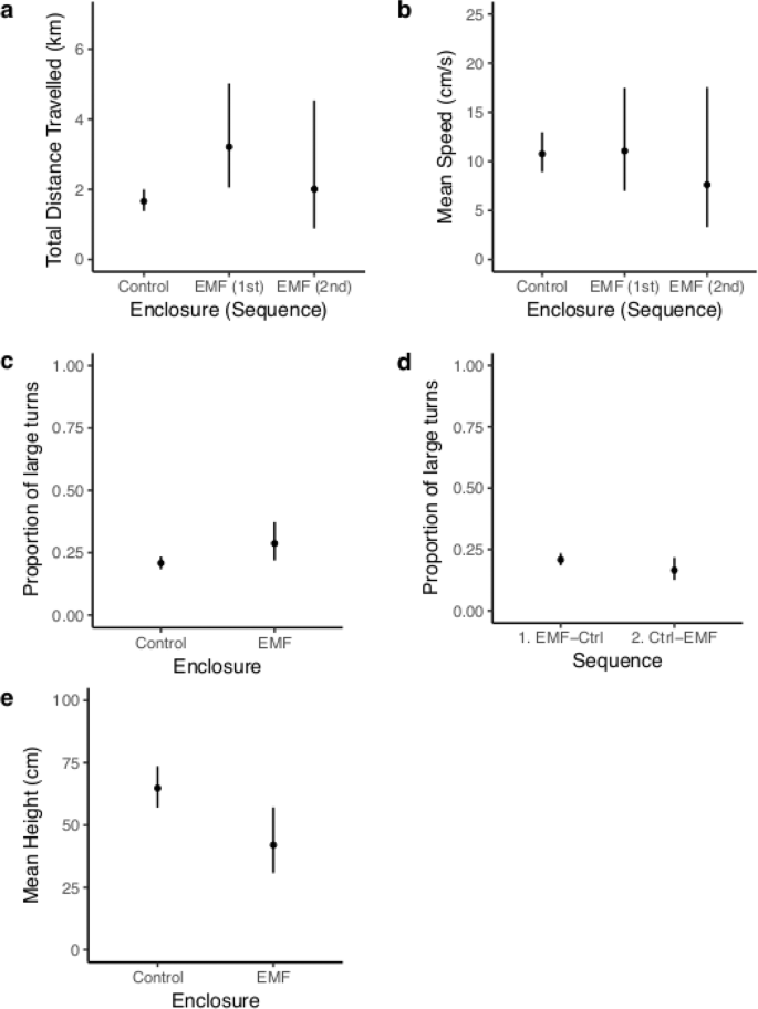
Skate behaviour in response to EMF. (a) The modelled estimates of the mean total distance travelled by skates in each enclosure as influenced by the sequence of exposure to the enclosures. (b) The modelled estimates of the mean speed of movement by skates at each enclosure as influenced by the sequence of exposure to the enclosures. (c) The modelled estimates of the mean proportion of large (170–180°) turns by skates at each enclosure; and for each sequence (d). (e) The modelled estimates of mean height of the skates from the seabed at each enclosure. The estimates were back-transformed where appropriate and the 95% confidence intervals are shown. The maximum EMF at the base of the treatment enclosure was 65.3 µT and the control enclosure was 51.3 µT.
Lobster behaviour
Significant differences were found in the proportion of large turns made by lobsters and their height from seabed when compared between the control and treatment enclosure with some influence of the sequence of exposure (Table 1). Distance: The mean total distance travelled by lobsters per day was similar at each enclosure with only 7% difference (Control: 4.05 km (95% CI; 3.75–4.35 km), Treatment: 3.76 km (95% CI; 3.13–4.38 km). Speed: The estimated mean speed of lobster movement at each enclosure was similar with only 3% difference (Control: 10.14 cm s−1 (95% CI; 9.06–11.34), Treatment 10.41 cm s−1 (95% CI; 8.28–13.10)). Proportion of large turns: The estimated mean proportion of large turns by control lobsters was 0.14 (95% CI; 0.11–0.17) while for treatment lobsters (1st in the sequence) it was 0.11 (95% CI; 0.07–0.17). The treatment lobsters showed a 16% lower proportion of large turns than control lobsters (Fig. 2a). For the treatment lobsters (2nd in the sequence), the proportion of large turns was 0.18 (95% CI; 0.08–0.23); a 34% higher proportion of large turns (Fig. 2a). Lobsters used an increased proportion of large turns at the enclosure second in the sequence of exposure, regardless of enclosure. However, this trend was stronger when the second enclosure was the treatment compared to when it was the control. Height: The estimated mean height of control lobsters from the seabed was 26.40 cm (95% CI; 25.06–27.81) while treatment lobsters were 22.65 cm (95% CI; 20.00–25.66) from the seabed (Fig. 2b). Treatment lobsters were closer to the seabed by 14%.
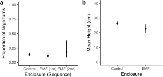
Lobster behaviour in in response to EMF. (a) The modelled estimates of the mean proportion of large (170–180°) turns by lobsters at each enclosure, as influenced by the sequence of exposure to the enclosures. (b) The modelled estimates of mean height of the lobsters from the seabed at each enclosure. The estimates were back-transformed and the 95% confidence intervals are shown. The maximum EMF at the base of the treatment enclosure was 65.3 µT and the control was 51.3 µT.
Comparing animal behaviour between enclosures and EMF zones
The cable crossed the enclosure, off-centre and at an 86° angle; approximately perpendicular to the long side. This presented a gradient of EMF within the treatment enclosure allowing two zones of high (>52.6 µT) and low (<49.7 µT) EMF to be spatially defined (Supplementary S3) and comparable spatial zones were defined at the control enclosure (both 51.3 µT). Statistically significant behavioural parameters (Table 1) were analysed to determine if animal behaviours were associated with high (>52.6 µT) or low (<49.7 µT) EMF (different zones; calculations were proportional to their aerial extent; Supplementary S3) at the treatment enclosure, by calculating the difference between zone 1 and zone 2, and comparing the difference between the two enclosures. Low EMF is caused by the magnetic field induced by the cable electrical current cancelling, in part, the Earth’s magnetic field, thus, lowering the total field.
Skate: Comparing between treatment and control enclosures indicated that the skates spent a greater amount of time in zone 1 (high EMF (>52.6 µT) at the treatment enclosure (n = 8, t = −2.366, df = 13.9, p = 0.033, Fig. 3a,b). Within the zone of high EMF the skates also travelled further (n = 8, t = −2.662, df = 13.6, p = 0.019; Fig. 3c,d) and exhibited a higher frequency of large turns (n = 8, t = −2.284, df = 14, p = 0.039; Fig. 3e,f). There was no significant difference in mean skate speed of movement (n = 8, t = 1.476, df = 9.8, p = 0.171) or the height from seabed (n = 8, t = 0.355, df = 9.0, p = 0.731).
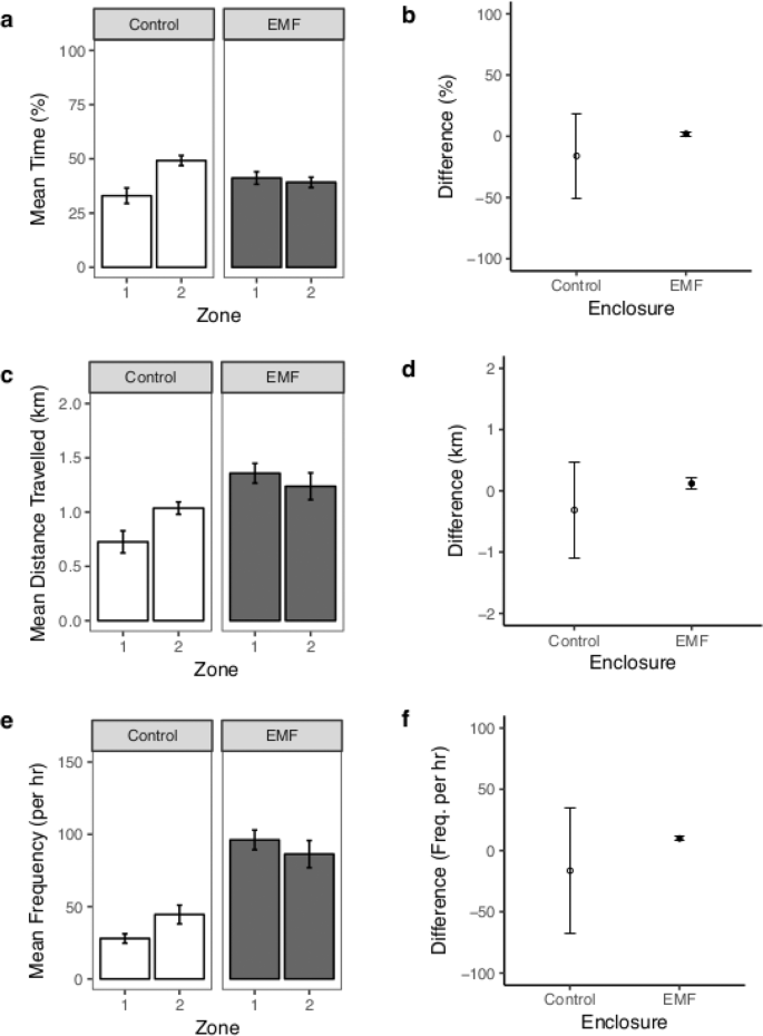
Skate behaviour in each zone of the enclosures. (a) The group mean (±SE) of the mean proportion of time skates spent in each zone (Zone 1 > 52.6 µT, Zone 2 <49.7 µT) at each enclosure, with (b) the arithmetic mean difference (±95% CI) in time spent in each zone (i.e. Zone 1- Zone 2) at each enclosure. (c) The group mean (±SE) of the total distance travelled per day by skates in each zone at each enclosure with (d) the arithmetic mean difference (±95% CI) in distance travelled in each zone at each enclosure. (e) The group mean (±SE) of the frequency of large turns per hour by skates in each zone at each enclosure with (f) the arithmetic mean difference (±95% CI) in the frequency of large turns per hour in each zone at each enclosure. Note, the comparison is firstly the difference between zone 1 and 2 in each enclosure and then between the enclosures.
Lobster: The proportion of large turns (n = 13, t = −0.479, df = 23.1, p = 0.636) and the height from seabed did not differ between zones within the enclosures (n = 13, t = −1.410, df = 21.7, p = 0.173).
Summary of animal behaviour in response to EMF
The results of this study clearly demonstrate that there were multiple statistically significant differences in the behavioural parameters assessed, when exposed to the EMF of the CSC, in both skates and lobsters. The basic comparison made is between the behaviour of animals in the control enclosure to the behaviour of animals in the treatment enclosure where they were exposed to an EMF from the cable. The analyses completed also account for the grouping structure and sequence of exposure to the two enclosures.
The assessment of spatial distribution patterns (Supplementary S2) showed that skates and lobsters both used the full extent of the enclosures, however, they spent significantly different periods of time in the central area of the two enclosures. The strongest behavioural response to EMF was found in the electrosensitive species, the Little Skate, where they were observed to differ significantly in the distance travelled per day, speed of movement, their height from seabed, and proportion of large turns. Furthermore, in the skates, the different pattern of spatial distribution, distance travelled and proportion of larger turns was associated with the zone of high EMF (>52.6 µT). These analyses are summarised for each skate behavioural parameter in Table 2. The lobsters, a putative magneto-sensitive species, also demonstrated statistically significant responses to the EMF, in the proportion of large turns and height from seabed. There was however no indication that either of these parameters were associated with zones of high or low EMF but was an overall response. The lobster analyses are summarised for each behavioural parameter in Table 3.
Enclosure EMF
The measured magnetic field is the result of a superposition of the Earth’s magnetic field and the cable-generated field, which introduces an asymmetry between the two sides of the cable (Fig. 4a). The peak magnetic field at the seabed (i.e. enclosure base) was 65.3 μT (max); a clear deviation from the Earth’s magnetic field (51.3 µT). The treatment enclosure was positioned at 94° relative to the cable direction. The peak fields at mid and top height of the enclosure were weaker (55 and 53.5 µT respectively). There was good agreement of measured and modelled (Supplementary S4) magnetic fields of the base, mid and top of the enclosure (Fig. 4b). The model (Supplementary S4) indicates that the two bundled cables were placed at 120° relative to the vertical direction, with 0.1 m separation. The burial depth was estimated to be 1.3 m (4.4 feet). The model reveals that the cable was positioned 0.25 m from the maximum magnetic field level towards the centre of the enclosure (Fig. 4b, vertical line). For comparison, animals at the control enclosure were exposed to ambient magnetic fields (51.3 µT).
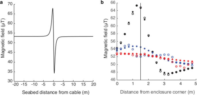
The measured and modelled magnetic field at the treatment enclosure. (a) The measured magnetic field of the CSC transect which was targeted for the treatment enclosure to be positioned. The maximum deviation of the Earth’s magnetic field was 18.7 μT. The electric current in the cable was 345 A. (b) The measured (open circles) and modelled (filled circles) magnetic field inside the enclosure. The optimization was done on the magnetic field measured at the seabed (black) and then modelled for the mid (blue) and top (red) of the enclosure. The long side of the enclosure starts a 0 m and ends at 5 m.
Electromagnetic Fields of HVDC cables
Variation in EMFs with electrical current
Measurements of the EMF were taken near to the seabed by sledging the sensors over the cable. For both the Cross Sound Cable (CSC) and Neptune Cable (NC) the DC magnetic field and an unexpected AC (magnetic and electric) field were detected. The variation in each field with the operating electrical current in the cable is described.
The CSC (highest nominal current 1175 A) was measured at a maximum of 345 A where the maximum deviation of the total magnetic field (DC), relative to the Earth’s magnetic field, was 18.7 µT (negative). The average deviation of the total magnetic field (DC) was considerably higher at 345 A than when the current was 16 A (Table 4). The average positive and negative deviation of the magnetic DC field at 345 A was 3.79 and 2.83 μT and at 16 A was 0.40 and 0.28 μT, respectively (Table 4). These observations show that electric current in the cable generates deviations comparable to the strength of the Earth’s magnetic field.
The average AC fields at 345 A were 0.15 μT (AC magnetic, Table 4) and 0.72 mV/m (AC electric, Table 4). These values were comparable to levels obtained at 16 A, which were 0.14 μT and 0.74 mV/m (Table 4).
During the CSC shut down (0 A), the average DC field was twice as weak as when the electric current was 16 A. The DC field was discernible, however, there was no sign of the AC field.
When the NC operated at full power, corresponding to 1320 A, the maximal deviation was 21 μT (positive). At 1320 A, the average positive deviation of the magnetic DC field relative to Earth’s magnetic field was 6.77 μT and the average negative deviation of the magnetic DC field was 2.3 μT (Table 4). At 660 A, the average positive magnetic deviation of the DC field relative to Earth’s magnetic field was 3.0 μT and the average negative deviation of the magnetic DC field was 0.9 μT (Table 4).
At 1320 A, the average magnetic AC field was 0.04 μT and the average electric AC field was 0.42 mV/m (Table 4). When the current was 660 A, the corresponding AC fields were 0.023 μT and 0.24 mV/m (Table 4).
Spatial extent, symmetry of signals and harmonics of the EMF
The DC magnetic fields typically extended 5–10 m on either side of the cable. As reported in Table 4, the magnitude of the positive and negative deviation of the total magnetic field (DC) differed and resulted in an asymmetrical field (Fig. 4 & Supplementary S5). This pattern is due to the rotation of the cable pair in the cable relative to the vertical axis.
Generally, the widths of the electric fields were larger than the corresponding magnetic fields. For example, in Fig. 5A the reduction of measured fields to 10% of the maximum field strength, was observed at approximately 8 m from the maximum for the magnetic field and 48 m from the maximum for the electric field. The AC fields were approximately symmetrical in shape. The frequency of the measured AC fields ranged from >1 Hz (i.e. extremely low frequency) to <2500 Hz, which is also the extent of the SEMLA’s sensitivity range for electric fields. In the CSC the dominating frequency for the magnetic AC field was 60 Hz, followed by 180, 540 and 120 Hz harmonics and for the electric AC field 540 Hz followed by 180, 900 and 60 Hz harmonics (Fig. 5b). The AC fields were detectable even when the cable was not transmitting power but had a maintenance current of 16 A (Fig. 5c); considerably higher than the background levels (grey Fig. 5b,c). In the NC the dominating frequency for both the magnetic and electric field was 720 Hz, followed by 120, 180 and 360 Hz harmonics.
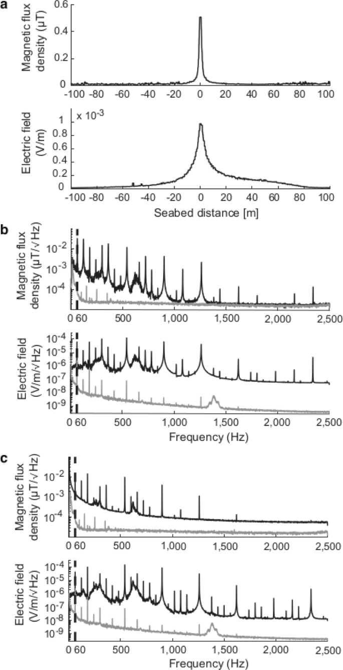
The spatial extent and harmonics of the AC fields, exemplified by the CSC. (a) The spatial extent of the measured AC fields; the total magnetic AC field (upper) and the total electric AC-field (lower). (b) The estimated spectra from the Power Spectral Densities (PSD for transect 7, black lines) during operation at 345 A; the magnetic field (upper) and the electric field (lower). The grey lines show measured background levels. (c) The estimated spectra from the PSD of transect 5 when the CSC was not transferring power but had an electric current of 16 A. In (b,c), the upper panel shows the magnetic AC field (black) and the lower panel the electric AC field (black). Both have the main frequency of 60 Hz identified by a dotted line and the grey lines in (b,c) show the background levels obtained at the reference site (358 m from the cable).
Electromagnetic field modelling
The previously described measured fields were not only affected by the magnitude of the transmitted electric current, but also by the morphological and structural properties of the cable, and the burial depth. Two models were successfully developed to describe the DC magnetic field. To accurately predict the fields at the seabed and in the water column, a model was implemented based on COMSOL software. This model made detailed estimates of the fields, based on cable geometry and material properties, in order to compare the modelled results with measured fields. The model was, however, computationally expensive and could not be used in iterative schemes. Therefore a fast model was developed based on simplified assumptions of the cable such as infinite length and no magnetic materials. The fast model was used in an optimization mode to predict the geometry and burial depth of the cable using the measured levels at the seabed and known electric current. The same model was specifically used in forward mode to estimate the EMF in the enclosure volume based on optimized parameters (Fig. 4b). Both models were accurately parameterized based on the need to describe the DC magnetic field of HVDC cables (Supplementary S4).
Using the fast model, the burial depth of the CSC (345 A) and the NC (1320 A) was estimated from the transect crossings at constant power. The estimated minimum burial depth achieved in the CSC transects was 0.58 m and the maximum 1.74 m (x = 1.41, sd = 0.37, n = 9). The estimated minimum burial depth of the NC transects was 1.16 m and the maximum 2.62 m (x = 2.09, sd = 0.35, n = 31).
Source: Ecology - nature.com

