Constraining size-dependence of vegetation respiration rates

Data collection for meta-analysis

Data used in the meta-analysis were obtained from two main sources – Internet searches on (1) Web of Science (Clarivate Analytics, Philadelphia, PA, USA) and (2) Google Scholar (Alphabet, Mountain View, CA, USA) – using keywords such as “autotrophic respiration”, “ecosystem”, “forest”, and “carbon cycle”. I collected original papers as much as possible and looked for data on ecosystem-scale autotrophic respiration, heterotrophic respiration, phytomass (plant biomass carbon stock), and soil organic carbon stock. I used observed annual values for respiration rates; to avoid extrapolation biases, daily to seasonal values were excluded. I also collected supplementary records from open-access datasets provided as part of several syntheses on the terrestrial carbon cycle^32,33,34. Here again, I consulted original papers as much as possible to reduce data-extraction errors.

I then developed a database comprising records from the literature (Supplementary Table S1). Several sites reported multiple values derived by using different assumptions and correction methods; these were included in the analyses to assess the range of uncertainty caused by data handling. For each record, I collected site information for ancillary analyses: site latitude, land-cover type, annual mean temperature, annual precipitation, plant individual density, stand age (mostly for forests), basal area, canopy height, leaf area index, and so on. For ecosystem-scale carbon stock and respiration, units were standardized to Mg C ha⁻¹ and Mg C ha⁻¹ yr⁻¹, respectively. Dry weight was converted to carbon weight by multiplying by a coefficient of 0.45; conversion from CO₂ weight to carbon weight was done by multiplying by 12/44. For several studies, total autotrophic respiration rate was obtained by summing component fluxes from plant organs; data that lacked major components (e.g., only aboveground respiration) were therefore not used.

Most respiration measurements in these studies were conducted by the chamber method. Specific respiration rates of vegetation components (e.g., leaf, stem, and root) were measured with cuvettes and then scaled up to ecosystem scale. Few direct measurements of whole-ecosystem autotrophic and heterotrophic respiration have been conducted at ecosystem scale because of practical constraints. Note that ecosystem-scale fluxes measured by the eddy-covariance method quantify net ecosystem CO₂ exchange only; photosynthetic assimilation and ecosystem respiration were then estimated from net fluxes by using appropriate separation methods such as non-linear regression.

Statistical analyses were conducted in SPSS Statistics v. 25 (IBM Inc., Armonk, NY, USA). To obtain 95% confidence intervals for the regression coefficients (e.g., scaling exponents in the form of power laws), bootstrapping was conducted 1000 times. The null model was based on the null hypothesis that vegetation respiration rate is independent of biomass (Supplementary Fig. S9).

Temperature correction of plant respirationrates

In general, the temperature response function, f(T), is described as:

where E_a is the activation energy (0.6 eV for metabolic rate), and k is Boltzmann’s constant (8.62 × 10⁻⁵ eV k⁻¹). The temperature response of plant (and microbial) respiration is often parameterized as an exponential function with a parameter Q₁₀ (increase per 10 °C temperature rise) as:

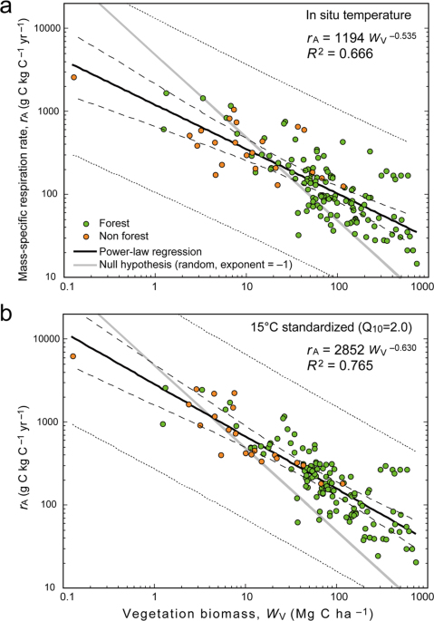
where T₀ is the base temperature (for example, 15 °C) at which f(T) takes the value 1. In many models, this function is applied to maintenance respiration, whereas the construction respiration is assumed to be proportional to growth rate. Thus, as a result of changes in maintenance and growth components, the apparent f(T) can change through time and between places. When standardizing the respiration rates obtained under different temperature conditions, the data were divided by f(T) values to convert them into the value at the base temperature, for example:

In Fig. 1b, a Q₁₀ value of 2.0 was used for this conversion. Moreover, as a result of thermal acclimation, Q₁₀ varies seasonally and geographically. The relationship between temperature and foliar respiration Q₁₀ has been summarized as follows²⁶:

Terrestrial model simulation outputs

Global simulation outputs of R_A and W_V were derived from the MsTMIP³⁵ dataset, available from https://daac.ornl.gov/cgi-bin/dsviewer.pl?ds_id=1225. This study uses outputs of 14 models, which provide data on autotrophic respiration and plant biomass at a spatial resolution of 0.5° × 0.5° in latitude and longitude. For carbon cycle models (GTEC, LPJ-wsl, ORCHIDEE, SiBCASA, VEGAS2.1, and VISIT), the results of the MsTMIP SG3 experiment were used. The models were driven by time-series data on atmospheric CO₂, climate, and land-use change. For carbon–nitrogen models (BIOME-BGC, CLASS-CTEM-N, CLM4, CLM4VIC, DLEM, ISAM, TEM6, and TRIPLEX-GHG), the results of the MsTMIP BG1 experiment were used. The models were driven by time-series data on atmospheric CO₂, nitrogen deposition, climate, and land-use change. For each model and cell, values of R_A and W_V were averaged for the period 1991–2010. When standardizing temperature at 15 °C, grid temperature was obtained from CRU TS3.2³⁶.

Plant trait TRY database

Values of r_A for different plant organs were downloaded from the TRY database²⁹ (https://www.try-db.org/TryWeb/Home.php; accessed 30 July 2019). This study used the following open access datasets: “Leaf respiration rate in the dark per leaf dry mass (trait no. 41)” (n = 10,719), “Root respiration rate per root dry mass (trait no. 514)” (n = 1161), and “Stem respiration rate per stem dry mass (trait no. 519)” (n = 540). These data were obtained by many different researchers for various plant species under different observational conditions. For each organ, the average, standard deviation, median, and 25% and 75% quartiles were calculated.

Global R _A estimation

The global value of R_A and its estimation range were obtained by applying the meta-analysis regression equation to the global map of vegetation biomass³⁷ (Fig. 4a). The calculation was conducted at approximately 1 km (30″ in latitude and longitude) resolution. Global total R_A was estimated as 64.0 Pg C yr⁻¹ by using the equation in Fig. 1a; a sensitivity analysis showed that it varies from 60.4 to 66.4 Pg C yr⁻¹ with a ± 10% change in biomass at each grid. The range of estimation uncertainty was obtained by perturbing coefficients in the regression equation: from the meta-analysis, standard deviations were 159.0 for the multiplier coefficient and 0.0358 for the exponent. Also, vegetation biomass was perturbed by ±10% standard deviation in each cell. Equation coefficients and biomass were randomly sampled 1000 times, and used independently for estimation of global R_A. Finally, the average and standard deviation were calculated.

Source: Ecology - nature.com