Contribution of land use to the interannual variability of the land carbon cycle

The bookkeeping and residual budget approach

In the IPCC AR5 (ref. ¹²) and the annual global carbon budget updates by the GCP (ref. ¹³), the S_net was derived using the following equation:

where S_net is the net land sink, E_FUEL is the CO₂ emissions from fossil fuel burning and cement production, S_AIR is the atmospheric carbon sink in the form of CO₂ growth for which reliable global measurements since 1959 are available, and S_OCEAN is the ocean carbon sink. All terms are defined as annual carbon fluxes. A positive sign of sink flux variables indicate removal of carbon from the atmosphere, while a positive sign of emission flux variables indicates release of carbon into the atmosphere. In this study, the fluxes of E_FUEL, S_AIR, and S_OCEAN for 1959–2015 were extracted from the Global Carbon Budget 2017 released by GCP (ref. ¹³).

We use the phrase net land sink for S_net because it is a net effect between two opposing terms: S_Intact subtracted by E_LUC from managed land:

where a positive sign of E_LUC indicates net release of carbon to the atmosphere. E_LUC occurs because relatively carbon-poor managed ecosystems replace carbon-rich intact ecosystems, and release their stored carbon into the atmosphere. S_Intact indicates carbon sink over land with no appreciable human modification and whose carbon sink can be mainly ascribed to global environmental changes, including atmospheric CO₂ growth, climate change, and nitrogen deposition.

While S_net can be relatively well constrained following Eq. (1) with reliable estimates for all terms on the right hand side of the equation, neither S_Intact nor E_LUC can be directly measured over a large area; modeling therefore serves as the principal approach for their quantification. To estimate E_LUC, bookkeeping models track over homogeneous geographical units the areas of forest loss and agricultural land gains, and subsequent abandonment, together with forest wood harvest and regrowth. Such land-use transition information is then further combined with carbon densities for various ecosystems, along with the temporal response curves of carbon pools after a land-use transition, to account for separately gross emissions, following land clearance and recovery sinks after agricultural abandonment and forest regrowth. In the IPCC AR5 and until the GCP annual carbon budget update for the year 2015 (ref. ¹⁴), E_LUC was predominantly estimated by the bookkeeping model of Houghton and colleagues^19,39, which was widely adopted by the carbon cycle community. Subsequently, S_Intact is estimated by rearranging Eq. (2) as:

In this approach, S_Intact is derived as a residual term of the carbon budget, and is often referred to as the residual land sink. In the current analysis, for carbon fluxes quantified using the bookkeeping and residual budget approach, i.e., following IPCC AR5 and ref. ¹⁴, we used the estimated E_LUC and its components from the most recent work by ref. ¹⁹ (hereafter shortened as HN2017), which includes large-scale historical deforestation and wood harvest (for details please refer to ref. ¹⁹) in land-use transitions. S_net and S_Intact were then calculated using Eqs. (1) and (3), respectively. Note that in the most recent global carbon budget by GCP (ref. ³²), S_intact was derived by a group of DGVMs forced by constant preindustrial land cover distribution with varying atmospheric CO₂, nitrogen deposition, and climate data. However, such S_Intact includes carbon fluxes over both managed and intact land today (rather than intact land only), and therefore the IAV of S_intact includes both managed and intact land as well, i.e., the separation of IAV in carbon fluxes between managed and intact land has not been done.

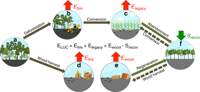
The HN2017 E_LUC estimate contains four different components according to the type of land-use transition involved and the time span over that the carbon flux occurs (main text Fig. 1): E_fire for immediate emissions following intact land clearance that often arise from burning of aboveground biomass residuals and other on-site disturbances, and are assumed to happen at the same year of clearance; E_wood for emissions from wood product degradation that extend over a long period after wood harvest; E_legacy for emissions over recently established agricultural land, resulting from the decomposition of slash and soil carbon as a legacy of former intact land; and S_recov for carbon sink in recovering secondary forest following agricultural abandonment or wood harvest. As such, E_LUC is quantified as:

The HN2017 bookkeeping model used fixed carbon densities and static temporal response curves of carbon stock change with time since land-use transition, and it was intended to include in E_LUC only the IAV due to changes in deforested area, but not those induced by climate variations and global environmental changes.

Improved ORCHIDEE model with sub-grid land cohorts

Another approach to quantifying E_LUC is to use DGVMs that run over spatially explicit grids and numerically incorporate physiological vegetation carbon cycle processes, including photosynthesis, carbon allocation, vegetation mortality, and litter and soil carbon decomposition. In most DGVMs, areas of different vegetation or plant functional types (PFTs) are represented as separate tiles or patches in a model grid cell, over which carbon cycle, energy, and hydrological processes are simulated. In the majority of them only a single tile is used for a given PFT, and consequently, for instance, carbon fluxes of intact forest and recovering secondary forest cannot be distinguished⁴⁰. This prevents them from estimating E_LUC by resolving each individual flux component in Eq. (4) as is done in bookkeeping models. Instead, for example, in most DGVMs that are used in the GCP annual carbon budget updates, E_LUC is derived from the difference between the S_net values in two parallel simulations: one with historical LUC and the other one without. Two features characterize such an approach: (1) compared with the E_LUC quantified using the bookkeeping method, E_LUC quantified by DGVMs includes the lost additional sink capacity that would otherwise occur in a world without any LUC but with atmospheric CO₂ growth; and (2) in terms of the IAV in E_LUC, IAV is dampened by subtracting carbon fluxes of two simulations that respond to climate variations in a symmetric way.

In this study, we used an improved version of the ORCHIDEE DGVM that is able to account for sub-grid cohorts for a given PFT that have different times since their establishment, so that the model has the strength to combine both bookkeeping functionality and the numerical representation of plant biophysics⁴⁰. The ORCHIDEE version used here has been extensively validated for northern regions⁴¹ and applied globally in the recent annual GCP carbon budget update¹³. In this improved version, the carbon balances of intact and managed land (e.g., intact forest and recovering secondary forest) can be completely separated. This capability allows the quantification of E_LUC and its individual components following Eq. (4), but with the advantage of accounting for the full impacts of environmental changes on E_LUC, and especially the impacts of climate variations.

Implementation of LUC. LUC processes shown in the main text Fig. 1 were implemented in ORCHIDEE in combination with the cohort functionality. For deforestation into agricultural land, intact forests were given a high priority to be cleared, reflecting the expansion of agricultural land in temperate regions over the history, and being consistent with the current-day agricultural expansion in the tropics. A certain fraction of aboveground biomass carbon was assumed as being released into the atmosphere within the same year as deforestation occurred, representing the common usage of fire for land clearing³³. Unburned biomass residuals and root biomass carbon were transferred to litter pool of the new agricultural land, whose decomposition with time contributed to legacy emissions. When agricultural abandonment led to forest recovery, young secondary forest cohorts were established and further moved to older forest cohorts with their growth, until being declared again as intact when their biomass exceeded a certain threshold. Transitions between natural grassland and agricultural land were handled in a similar approach, except that all biomass carbon stocks were transferred to the litter pool (i.e., no fire-induced immediate carbon emissions), and higher priority was given to young cohorts in both conversions of grassland to agricultural land and agricultural abandonment into grassland. Due to a lack of savanna vegetation type in ORCHIDEE, land-use transitions involving savanna were integrated into those of forest and grassland. Because transitions between any pair of land-use types were explicitly represented in ORCHIDEE, the spatial-scale nature of LUC activities was independent of the spatial resolution of the model simulation, but depended on the input LUC forcing datasets (refer to Supplementary Note 6 for detailed discussions).

For both industrial and fuel wood harvest, we started from intact forests and then move to younger cohorts in order to fulfill the prescribed annual-harvested wood biomass in the forcing data. This is consistent with the approach used in HN2017. For fuel wood harvest, the aboveground woody biomass carbon was assumed being emitted into the atmosphere during the same year as harvest occurred, whereas small branches and leaves were moved to litter pool. In the case of industrial wood harvest, certain fractions of aboveground woody biomass were stored as two wood product pools with a 10- and 100-year residence time, respectively, while the unharvested branches and leaves, and root biomass were moved to litter pool. Following harvest, young forest cohorts were planted and underwent the same process as secondary forests generated by agricultural abandonment.

Simulation setup. Comparing E_LUC and its components estimated by ORCHIDEE and by HN2017, provided that they were driven by shared LUC reconstructions and follow the same LUC parameterizations, allows us to elucidate the IAV of E_LUC and its contribution to the IAV of S_net. We first performed a baseline ORCHIDEE simulation to include the same LUC processes as in HN2017. These include large-scale processes, such as deforestation, afforestation/reforestation, and transitions between natural grassland and agricultural land, and wood harvest. For both ORCHIDEE and HN2017 estimates, the simulations were started from the year 1700, but the E_LUC was examined for the period of 1850–2015. The ORCHIDEE baseline simulation was driven by variable atmospheric CO₂ and CRUNCEP climate data at a 2-degree resolution (prior to 1901 climate data for 1901–1920 were recycled). Historical forest area changes and wood harvest biomass were driven by exactly the same data used in HN2017 for different geographical regions of the world (see Supplementary Figs. 1 and 2; more details are provided in Supplementary Note 1). Gridded annual agricultural area changes were derived from the LUH2 dataset⁴². When agricultural area changes could not be matched by changes in forest imposed by HN2017, they were implemented as transitions with natural grassland. To ensure the comparability with the HN2017 bookkeeping model, we implemented the same LUC parameterizations in ORCHIDEE. Please refer to Supplementary Table 1 for details in association with various E_LUC flux components.

Shifting cultivation is a local-scale subsistence agricultural practice that involves conversion of forest or natural grassland into agricultural land, maintaining such agricultural land for a certain period, and then setting it as fallow and repeating the whole cycle. Despite its existence as an early form of human land use and being active in certain regions of the tropics today, the areas subjected to shifting cultivation were of great uncertainty⁴³. Several DGVMs reported additional carbon emissions by further accounting for shifting cultivation, but its exact contribution to the global land carbon balance remains elusive⁴⁴. For these reasons, shifting cultivation was not included in the HN2017 study, or the ORCHIDEE baseline simulation for consistency purpose. Nevertheless, for the purpose of uncertainty analysis of our baseline results, we performed an additional sensitivity simulation accounting for shifting cultivation starting as early as 1500 (the SC-sensitivity run). Historical areas subjected to shifting cultivation between forest (or grassland) and agricultural lands were extracted from the LUH2 data⁴² (see Supplementary Note 2 for details of shifting cultivation implementation in ORCHIDEE), while all other drivers were the same as the baseline simulation.

To balance between computing resources demand and accurate representation of land management status, six age cohorts were used for forest PFT and two age cohorts were used for herbaceous PFT (i.e., grassland, cropland, and pasture) in the ORCHIDEE simulation. The results indicated that intact forest and grassland, permanent agricultural land (pasture and cropland) existing prior to 1700, and agricultural land established after 1700 (post-1700 agricultural land), as well as recovering secondary forest and grassland were well separated throughout the simulation (Supplementary Figs. 3 and 4). Two herbaceous PFT cohorts represented permanent and post-1700 agricultural land, or intact and recovering grassland, respectively. The management status of forest related to either disturbance history or recovery status. Before the start of the simulation, all forests were considered as intact in the baseline simulation (the uncertainty of this assumption was tested in the SC-sensitivity run). As time evolved, forest age structure changed (Supplementary Fig. 4). As a first approximation, we considered old-growth secondary forests as intact forests, when their wood mass exceeded 90% of the maximum attainable wood mass determined under preindustrial conditions. This roughly corresponded to a forest age of 70, 90, and 160 years for tropical, temperate, and boreal forests, respectively. Such age thresholds were consistent with the reported secondary forest ages that reached a similar status as intact forests from field investigations⁴⁵. To maximize the consistency with the HN2017 study, we further adjusted the composition of global intact and secondary forests, according to the HN2017 bookkeeping model at the end of the baseline simulation (i.e., 81% primary versus 19% secondary forests for the year of 2015, see Supplementary Note 4).

Model validation. The ORCHIDEE model was rigorously validated against observations to ensure a correct estimate of E_LUC in this study (for details see Supplementary Note 3). To properly simulate deforestation emissions, the spatial distribution of modeled aboveground biomass and deforestation area were compared with satellite observations (Supplementary Figs. 5 and 6). To capture secondary forest recovery, a database of forest biomass growth was constructed based on chronosequence observations. Modeled biomass–age relationships were then evaluated against this database for different forest types (Supplementary Fig. 7, Supplementary Table 2). Different from bookkeeping models, ORCHIDEE DGVM can account for global environmental changes and simulated forest carbon sinks can thus be compared with regional forest inventory data (Fig. 3). A top-down estimate of S_net could be reliably derived as a residual of carbon emissions minus sinks by the atmosphere and the ocean, both of which were based on observations. The magnitude and IAV of the simulated S_net, and its sensitivity to tropical land temperature variation were compared with the observation-based S_net derived by the residual approach (Figs. 6a, 7a).

Posttreatment of ORCHIDEE simulation: The S_net is defined as the simulated net biome production (NBP) over the globe, and is equal to net primary production after subtracting heterotrophic respiration, fire CO₂ emissions, and agricultural harvest. A positive NBP indicates carbon absorption by land. The NBP over intact forest and grassland was quantified as S_Intact. For the E_LUC flux components, E_fire and E_wood in Eq. (4) can be easily identified in ORCHIDEE. We treated NBP over secondary forest and grassland (being net primary production less heterotrophic respiration and fire carbon emissions) as S_recov, and the opposite of NBP over agricultural lands (croplands and pastures) as E_legacy. We assumed that NBP over recently established agricultural land was dominated by the decomposition of legacy slash and soil carbon, originating from former intact land. Note that the E_legacy in ORCHIDEE also included carbon fluxes over permanent agricultural land existing prior to 1700. Its scope was slightly different from the bookkeeping approach, where only post-1700 agricultural lands were included. But such a definition was coherent with our research objective to investigate the role of all lands under human land use in driving the IAV of S_net. Because permanent agricultural land showed only a small sink with very low IAV, its influence on the magnitude and IAV of E_LUC was negligible (Supplementary Fig. 10).

Attribution of IAV in S _net

S_net shows large IAV with temperature sensitivity providing a constraint on the magnitude of future climate–carbon cycle feedbacks. Following Eq. (2), to examine the IAV of S_net and attribute it to the effects of managed versus intact land, the temporal variance of S_net (Var (S_net)) was decomposed into the variances of E_LUC, S_Intact, and their covariance (main text Fig. 6d):

We also calculated the tropical temperature sensitivity of S_net ((gamma _{{mathrm{LAND}}}^{rm{T}})), S_Intact ((gamma _{{mathrm{Intact}}}^{rm{T}})), and E_LUC ((gamma _{{mathrm{ELUC}}}^{rm{T}})) as a way to infer climate–carbon cycle feedbacks (main text Fig. 7) for various land carbon fluxes. Tropical land air temperature anomalies were derived from the CRUNCEP climate data that forced the ORCHIDEE simulation, after removing the linear trend. Carbon flux anomalies were regressed against temperate anomalies using the ordinary least-squares linear regression, with the γ values given by the regression slopes.

Source: Ecology - nature.com