The results of the superposition of the LST and terrain factors
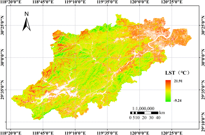
The natural LST information of the study area was obtained by using a radiative transfer model combined with the maximum likelihood method (Fig. 5). As seen from Fig. 5, although the high-temperature areas of the built-up lands (associated with frequent human activities) and low-temperature water bodies are essentially removed, the high LST values in autumn and winter are still mainly focused around the built-up lands, and the LST shows a significant cooling trend in the natural land surface environment near the woodlands.
available at https://support.esri.com/en/products/desktop/arcgis-desktop/arcmap/10.0.
Natural LST data of the study area without interference factors. Map has been created with ESRI ARCMAP 10.0,
Elevation, slope, and aspect and the shaded relief factor were extracted from the ASTER GDEM data (Fig. 6), the raster data (such as LST and terrain factor) were quantitatively processed, and the results were derived in numerical form to obtain the LST and terrain information corresponding to specific locations in the research area. A regression analysis was carried out by statistical methods, and the quantitative relationships between the variables were obtained by drawing a scatter diagram and data fitting.
Terrain factor extraction results. (a)–(d) Extraction results for elevation, slope, aspect and the shaded relief map. Maps have been created with ESRI ARCMAP 10.0 + ENVI4.8/IDL8.0,
Single-factor analysis of the terrain effect on LST
Correlation between LST and elevation
In this study, the correlation between LST and elevation data was discussed. A scatter diagram was drawn to obtain the results, as shown in Fig. 7. Figure 7a is the scatter diagram of the LST and elevation, and Fig. 7b is the scatter diagram of the LST and elevation excluding the artificial environmental disturbances, such as water bodies and built-up lands. The results show that there is a negative correlation between the LST and elevation, which is consistent with the results of existing research51.
Figure 7 shows that regardless of whether artificial environmental interference factors exist between the LST and elevation, there is an obvious trend that LST decreases gradually with increasing elevation. The regression analysis shows that the significance level in both cases is less than 0.01, and the linear regression relationship is obvious. The model correlation coefficient (R) in Fig. 7a is 0.551, and in Fig. 7b, it is 0.523. Based on this, when the effect of interference is removed, the LST of the study area decreases by approximately 5.16 °C for every 1 km rise in elevation. When interference is removed, the LST decreases by approximately 4.46 °C for every 1 km rise in elevation. That is, the comprehensive LST, including the artificial environment, declines faster with elevation than the LST in the natural environment, indicating that the comprehensive LST may change more significantly with elevation.
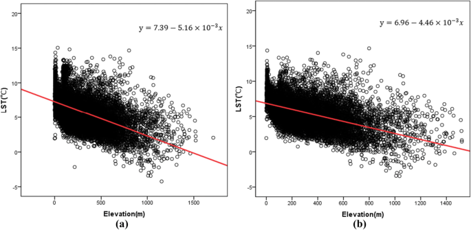
Regression analysis of the LST and elevation in the study area. (a) The results of the regression analysis between the LST and elevation. (b) The results of the regression analysis between the LST and elevation without interfering factors.
The main reasons for the influence of elevation on the LST are as follows. On the one hand, the influence of elevation on LST is mainly caused by air temperature, and the temperature value gradually decreases with increasing elevation. This pattern is observed mainly because the higher the troposphere atmosphere is from the ground, the less long-wave radiation energy it absorbs. The less heat the atmosphere stores, the lower the temperature is. However, the air temperature near the land surface shows a regular downward trend with increasing elevation, which in turn affects the heat exchange process between the surface and the air and finally acts on the surface heating processes16. On the other hand, considering the areas with higher elevations and larger topographic fluctuations, there are fewer human activities. That is, there are fewer anthropogenic disturbances, reducing the contribution of anthropogenic heat emissions to LST. Moreover, in this study area, the surface coverage at higher elevations is generally higher, and the cooling effect of green spaces makes the LST decrease with increasing elevation1,52,53.
Correlation between LST and slope
In this study, the slope in the terrain model was divided into eight ranges: 0°–10°, 10°–15°, 15°–20°, 20°–25°, 25°–30°, 30°–35°, 35°–40° and > 40°. The charts of the slope and LST statistical analyses were created according to the corresponding slope grades (Fig. 8).
As shown in Fig. 8, LST generally follows a gradually declining trend with increasing slope. Figure 8a, b represent the statistically derived results of LST (including the artificial environment and natural LST without interfering factors, respectively) and slope. The median, minimum and third and fourth quantiles of the LST in each slope range mostly follow the abovementioned pattern; the maximum value deviates slightly but does not have a major impact on the overall trend.
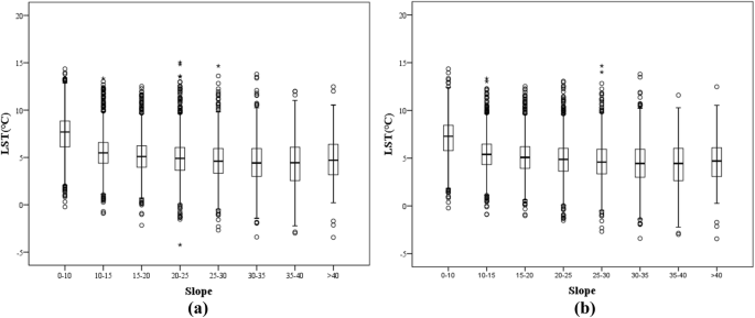
LST results of different slope ranges in the study area. The upper and lower black lines represent the maximum and minimum values, respectively. The third and fourth quantiles are represented by the upper and lower boundaries of the rectangle, respectively. The black line inside the rectangle represents the median, and the dots represent the outliers. (a) The statistical results of LST and slope, and (b) the statistical results of LST and slope without interfering factors.
A scatter diagram of slope and LST was created (Fig. 9) to further analyze the quantitative relationship between LST and slope. The results of the linear regression analysis show that the significance level between the two variables is less than 0.01, indicating an obvious linear relationship. The model correlation coefficient (R) in Fig. 9a is 0.537, and in Fig. 9b, it is 0.483. The results show that when the effect of interference on the LST and slope is removed, the LST decreases by 0.6 °C for every 5° increase in slope. When the disturbance factors (i.e., water bodies and built-up lands) are removed from the study area, the LST decreases by 0.5 °C for every 5° increase in slope. Therefore, slope is related to LST, and the steeper the slope is, the lower the LST. Many studies have shown that different slopes affect the temperature of surface objects by influencing the incidence angle and reflectivity of solar radiation54. Of course, in the process of temperature inversion, the presence of slope will often affect the angular relationship between the sun, the surface and the sensor; each surface will be affected by the reflection from adjacent surfaces55, which is one of the reasons why slope affects the LST.
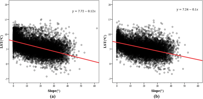
Regression analysis of LST and slope in the study area. (a) The results of the regression analysis between LST and slope. (b) The results of the regression analysis between LST and slope without interfering factors.
Correlation between LST and aspect
In this study, the aspect was divided clockwise into the northern (N) slope, northeastern (NE) slope, eastern (E) slope, southeastern (SE) slope, southern (S) slope, southwestern (SW) slope, western (W) slope and northwestern (NW) slope. The correlation between aspect and LST was explored by drawing statistically based charts (Fig. 10). Figure 10a represents the comprehensive statistical results of the analysis between aspect and LST, including the influence of the artificial environment. Figure 10b shows the statistical results of the analysis between the natural LST and aspect, without the influence of interference factors. This analysis shows that there were high values of LST on the eastern slopes, southeastern slopes, southern slopes, southwestern slopes and western slopes, and peak values typically appear near southern slopes.
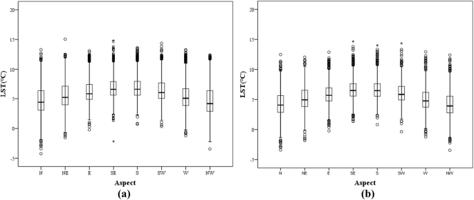
Statistical results of the analysis of the LST of different aspects in the research area. The upper and lower black lines represent the maximum and minimum values, respectively. The third and fourth quantiles are represented by the upper and lower boundaries of the rectangle, respectively. The black line inside the rectangle represents the median, and the dots represent the outliers. (a) The results of the statistical analysis between the LST and aspect, while (b) The results of the statistical analysis between the LST and aspect without the influence of the interfering factors.
Further, a scatter diagram of aspect and LST was drawn, and the quantitative relationship between these factors was analyzed. The results are shown in Fig. 11. The regression analysis showed that in both cases, the significance of the result was less than 0.01, indicating that the model has significant meaning. The model correlation coefficient (R2) in Fig. 11a is 0.115, and in Fig. 11b, it is 0.162. The correlation is not obvious. However, the results do generally explain the trend of high temperatures on the southern slopes and low temperatures on northern slopes. This is consistent with existing conclusions that sunny slopes receive more direct solar radiation, resulting in high slope temperatures and intense evaporation56. In addition, northern slopes are mostly associated with shaded low-temperature areas in the terrain, which is also one of the reasons for the abovementioned trend.
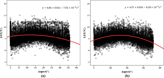
Regression analysis of LST and aspect in the study area. (a) The results of the regression analysis of LST and aspect. (b) The results of the regression analysis of LST and aspect without the influence of the interfering factors.
Correlation between the LST and values of the shaded relief map
Due to the influence of terrain fluctuation, when direct sunlight is partially or completely blocked and cannot reach a target, shadows will be formed in remote sensing images57,58. This work used the values of the shaded relief map to obtain information about the shaded geomorphology in the study area. Shaded relief is a cartographic technique that provides an apparent three-dimensional configuration of the terrain on maps and charts by use of graded shadows that would be cast by high ground if light were shining from the northwest. And it is the cosine of the sun incident angle and used in topographic correction method59,60,61,62,63. It can be calculated from the Topographic Model of the software ENVI. A value of 0 indicates that the corresponding pixel is almost completely covered in shadow64. A scatter diagram was drawn, and the correlation between the values of the shaded relief map and LST was quantitatively discussed with the addition of linear regression. The obtained results are shown in Fig. 12. Figure 12a represents the regression analysis results for the LST and values of the shaded relief map, and Fig. 12b represents the regression analysis results for the LST and shaded relief map without the influence of interfering factors. Studies have shown that the LST is positively related to the values of the shaded relief map, i.e., there is a negative correlation between the LST and shadows. Areas with greater coverage by shadows have lower LSTs. This is consistent with the previously reported trend that the shaded area has a lower LST due to the lack of sunlight and the accumulation of less solar radiation energy.
According to the regression analysis results, the model correlation coefficient (R) in Fig. 12a is 0.432, and in Fig. 12b, it is 0.482. The significance level of both is less than 0.01, so the results of the established model are significant. In addition, the removal of the disturbance factors has a certain influence on the quantitative relationship between the LST and values of the shaded relief map. By comparison, the LST changes more obviously with shadow topography under natural land surface conditions. It is believed that because the study area is in the Northern Hemisphere, the solar elevation angle in winter is smaller than that in summer, and the area in shadow on the remote sensing images is larger in the winter. In addition, compared with built-up lands, shadows in natural environments are mostly generated by rolling mountains, which leads to larger areas being covered by shadows, making the terrain effect more obvious.
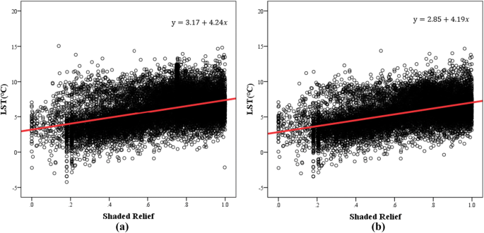
Regression analysis of the LST and values of the shaded relief map in the study area. (a) The results of the regression analysis of the LST and values of the shaded relief map. (b) The results of the regression analysis of the LST and values of the shaded relief map without the influence of the interfering factors.
Diverse analysis of the terrain effect on the LST
The research on terrain factors includes elevation, slope, and aspect and shaded relief maps. Through the regression analysis of each terrain factor and the LST, it is found that the abovementioned topographic features are correlated with LST. They affect surface water and heat distribution patterns and remote sensing imaging processes by changing the path of light propagation55,65,66. However, in reality, the effect of topography on LST is usually not determined by a single topographic factor, and the regional difference in LST is often the result of the comprehensive influence of multiple topographic factors. Therefore, only by comprehensively considering the effects of topography, such as elevation, slope, aspect and shaded relief maps, can the actual effect of topography on the LST be effectively described.
Based on the results of the correlations between each topographic feature and the LST, a multiple regression analysis of the topographic factors and LST was conducted. A stepwise method was used to establish the related variables in the model, and the best fit model was the one in which all four types of terrain factors were considered. Therefore, LST is set as the observable variable (y), and it is assumed to be affected by nonrandom factors, such as elevation (({x}_{1})), slope ({(x}_{2})) and aspect (({x}_{3})) and the shaded relief values ({(x}_{4})). The unknown parameters are denoted as ({beta }_{0}), ({beta }_{1}), ({beta }_{2}), ({beta }_{3}) and ({beta }_{4}), so the multiple linear regression model can be written as:
$$mathrm{y}={beta }_{0}+{beta }_{1}{x}_{1}+{beta }_{2}{x}_{2}+{beta }_{3}{x}_{3}+{beta }_{4}{x}_{4},$$
(6)
The unknown parameters were estimated by a least square method to minimize the error sum67. The significance of the regression equation and regression coefficient and the goodness of fit of the model were tested, and the results are shown in Table 2.
As Table 3 shows, the significance levels of the regression equation and regression coefficient are less than 0.01, indicating that the linear relationship between the variables is obvious. The quality of the multiple linear regression model can be measured by the complex correlation coefficient (R), coefficient of determination (R2), corrected coefficient of determination (({R}_{alpha }^{2})) and root mean square error (RMSE). In this regression model, the complex correlation coefficient (R) is 0.706. These statistical results indicate that there is a close linear relationship between the independent variables and dependent variables68. The coefficient of determination and corrected coefficient of determination (R2) are both 0.498, indicating that the established model has a good fit. The RMSE is approximately 1.529, which reflects that the established model will have relatively high accuracy for predicting the values of the dependent variables. In conclusion, the results support the use of linear regressions to study the effects of diverse terrain on LSTs. Elevation, slope, aspect and the shaded relief values tend to have a comprehensive effect on LST. Finally, the multiple linear regression equation obtained from the nonstandardized coefficient is:
$$mathrm{y}=4.996-0.003{x}_{1}-0.037{x}_{2}-0.001{x}_{3}+3.650{x}_{4},$$
(7)
where y is the LST (°C) and ({x}_{1})–({x}_{4}) represent elevation (m), slope (°), aspect (°) and the shaded relief value, respectively.
According to the optimal regression equation, among the influencing factors of terrain on LST, the shaded relief value contributes significantly more than the other factors and is positively correlated with LST. This indicates that compared with elevation, slope and aspect, the shaded relief value plays a decisive role in affecting the LST in the study area, which cannot be ignored in similar subsequent studies.
Although Hangzhou is an important starting point for us to choose to show the relevant experimental results. However, in order to verify whether the above conclusions are only a special case of Hangzhou, we selected additional a remote sensing image in Zhejiang Province which are different from the location of the study area in this paper for supplementary experiments. The data are processed in the same way as the original experiment. After the regression analysis of shaded relief factor, it is found that the LST increases gradually with the increase of shaded relief value. The significance level was less than 0.01, and the correlation coefficient R was 0.593. This not only shows that the model established on this basis has good applicability, but also preliminarily shows that it plays a decisive role in the above topographic factors.
Then a comprehensive regression analysis was carried out between the above topographic factors and LST. This step-by-step method is used to establish the relevant variables of the model. When the four types of terrain factors are considered, the model fits best. Through the test of the significance of the regression equation and regression coefficient and the goodness of fit of the model, it is found that the coefficient of the independent variable slope forward in the regression model is 0.000. This may be because the slope direction accounts for very little in the comprehensive effect of topographic factors and does not play a major role in the changing trend of the overall surface temperature. Therefore, the diversified terrain effect of removing the slope component is further considered in the study, and the multivariate regression linear equation composed of the following non-standardized coefficients is obtained
$$mathrm{y}=12.245+0.001{x}_{1}-0.032{x}_{2}+4.995{x}_{3},$$
(8)
In the formula, y is the LST (°C), and ({x}_{1})–({x}_{3}) represent the elevation (m), slope (°) and the shaded relief value, respectively. And the complex correlation coefficient R of the model is 0.616, which shows that the model has a certain practical application. However, no matter how the model changes, the, shaded relief factor plays a decisive role in the land surface temperature in the above topography. The supplementary experimental results further enhance the credibility of the original experimental results, indicating that the core results in this paper are not limited to Hangzhou area, its applicability in other area and images has been verified.
Source: Ecology - nature.com
