Data-driven modelling and spatial complexity supports heterogeneity-based integrative management for eliminating Simulium neavei-transmitted river blindness

Data

The data used in this study were collected from sentinel field sites in three onchocerciasis endemic foci in western Uganda, viz. Itwara, Kashoya Kitomi, and Bwindi, as part of the monitoring and evaluation activities associated with the Ugandan Onchocerciasis Elimination Program (UOEP). While onchocercal transmission foci can extend to a range of distances from the fly source rivers, the sentinel villages for monitoring the impacts of interventions in Uganda are normally selected among those closest to these rivers to ensure that communities with the highest prevalence are longitudinally monitored to reflect impact in likely worse-case settings within a focus⁴⁵. Note that while this design is efficient for monitoring the effects of an intervention in a focus, it will also reduce the potential extent of between-site infection/transmission heterogeneity among the chosen sentinel sites investigated in this work as compared to villages chosen randomly throughout the spatial extent of each focus.

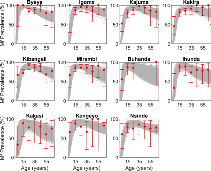
Altogether, data assembled from sixteen such sites were selected for use in the present analysis based on the variable availability of baseline and follow-up microfilariae (mf) prevalence data, focus-level black fly annual biting rate (ABR) data at baseline, and details of interventions applied in each focus (Table 1 and Supplementary Table S7). Of these sites, eleven were from the hyperendemic Itwara and Kashoya Kitomi foci. The baseline mf prevalence in these villages ranged from 76.3% to 92.1%, and the black fly species responsible for transmission of Onchocerca volvulus in both foci is Simulium neavei. Note, however, that follow-up monitoring data from 2004 were available for only six of the sites (Table 1).

Initially, control efforts in these foci and across Uganda relied solely on annual rounds of community directed treatment with ivermectin (CDTi), but efforts were then scaled up to include vector control⁶⁶. Successful elimination of the vector from several foci in Uganda using ground applications of temephos (Abate) eventually also shifted the focus of the program to transmission elimination rather than just control⁶⁶. Thus, control activities in the Itwara focus specifically included 19 rounds of annual mass drug administration (MDA) with ivermectin from 1991–2009, with inclusion of vector control by ground larviciding at intermittent periods beginning from mid-1995 – June 2003^56,67. In the Kashoya Kitomi focus, annual MDA with ivermectin began in 1991 and continued through 2006. In 2007, control efforts in this focus transitioned to biannual MDA, which continued through 2013 (Table 1). Vector control by ground larviciding was implemented here in July 2007 – October 2010⁶⁸. Site-specific MDA coverage observed for the six villages from these foci that have follow-up data are given in Supplementary Table S7.

Impacts of vector control were investigated by UOEP by measuring changes in the aggregate values of ABR in each focus. Typically, biting data from human landing catches (HLCs) carried out in 14 catching sites along the relevant river system in a focus during the 4-5 months pertaining to the major transmission season (at frequencies of 2 days per week) were used to make these focus-level ABR calculations using the calculation methods described in⁶⁹.

In addition, five villages from Bwindi, most of which are hypo- and mesoendemic, were also included in this study to consider a more heterogeneous sample of sites in the analyses (Table 1). For these sites, baseline mf infection data are aggregated at the community level and there was no biting rate information available (Table 1), requiring us to use model fits to the mf prevalence data to estimate the corresponding ABR information. Transmission here is also mediated by S. neavei, and both MDA and vector control interventions were carried out in this focus (Supplementary Table S7).

The Onchocerciasis transmission model

The onchocerciasis transmission model used here is an immigration-death ecological model describing population level parasite transmission dynamics in both the human and black fly hosts. The general structure of the model follows that incorporated in previous deterministic population models of onchocerciasis transmission and control dynamics^{47,70,71,72,73,74,75}, although here we develop and include functions describing the population-averaged mf uptake and larval development in the vector as well as the operation of different forms of host immunity in populations, while model implementation is carried out within a Bayesian Monte Carlo data-model assimilation framework that facilitates the simultaneous incorporation of information regarding local transmission parameters from data and assessment of the impact of uncertainty in the values of these parameters on model outputs^{31,38,49,50,76,77,78}.

Technically, the present model is based on a hybrid coupled partial and ordinary differential equation system, where the population-level age-structured pre-patent (P) and patent (W) worm burdens, microfilarial counts (M) (mf/mg of skin), and acquired immunity level (I) in the human host are dynamically modelled by a set of partial differential equations over time (t) and age (a), whereas the dynamics of infective stage L3 larvae (L) in vector hosts (simuliid fly populations) are modelled by an ordinary differential equation over time. To reflect the significantly faster time-scale of the infection dynamics in the vector hosts, we, however, make the simplifying assumption that the density of infective stage larvae in the vector population reaches a dynamic equilibrium rapidly (L*)^70,75. The governing equations of this model are:

Apart from multiple interacting components, complexity in the model is also governed by the operation of several density-dependent functional forms (denoted by the terms F_x) that moderate the transitions or development rates of different stages in the parasite’s life cycle. These regulatory processes underpin the operations of two forms of host immunity, namely acquired immunity to incoming larvae (F₁[I(a,t)]) and host immunosuppression by existing infection (F₂[W_T(a,t)]), mf production by patent worms (F₃[W(a,t)]), and the development of infective stage larvae in the vector (F₄[M(a,t)]). The larval death rate (σ_L) and excess vector mortality (σ_e) due to infection⁴⁷ are also both considered in F₄. Note that some functions are dependent on the total worm load where W_T = W(a,t) + P(a,t), while others depend on larval states (L*) and host immunity (I). To capture the effects of worm patency, we consider that at any given time t, human individuals of age less than or equal to pre-patency period, (tau ,) will have no adult worms or microfilariae, ie. W(a,t) = M(a,t) = 0 for a ≤ τ, and the rate at which pre-patent worms survive to become adult worms in these individuals at a > τ is given by (zeta ={e}^{-{mu }_{W}tau }). The establishment rate of larvae in the human host, represented as Φ, is moderated by effects of acquired immunity (as modelled by function, F₁[I(a,t)]) and/or immune tolerance (modelled by function, F₂[W_T(a,t)])^73,74. Given that previous modelling studies have underscored the potential for the involvement of either or both acquired immunity and immunosuppression in filarial infections^47,73,75, we include both these types of immunity in our model; however, we do not make any a priori assumptions concerning their occurrence in a particular study site but instead use the mf prevalence data to determine the operation of each or both in a site (see discussion of data-assimilation using the Bayesian Melding framework below). The mathematical representation of adult Onchocerca volvulus worm mortality has recently been a topic of discussion⁷; here, we use a constant mortality rate following the example of Basañez and Boussinesq⁴⁷ and Filipe et al.⁷⁵. The vector biting rate (λ, a parameter in the function Φ) in this model considers the number of bites per black fly to be equal to the human blood index (H_b) divided by the gonotrophic cycle (g). All model parameters and their descriptions are given in Supplementary Table S8. The respective density-dependent functions expected to modify or regulate transmission are given in Supplementary Table S9.

Species-specific microfilariae uptake and L3 larval development

There exists a non-linear relationship between the uptake of mf by the black fly and the resulting L3-stage larval load⁷⁹. This relationship will be dependent upon whether or not the relevant black fly species has developed cibarial armature, which we capture in the establishment rate term f[M(a,t)]. Following facilitation and limitation model formulations we developed previously³², the population-level mf uptake and larval establishment rate function for black flies with cibarial armature can be written as:

whereas for black flies without developed cibarial armature we used the form:

In the above, (k={k}_{0}+{k}_{Lin}M) is the shape parameter of the negative binomial distribution on the mf uptake whereas r and κ are respectively the rate of initial increase and the maximum level of L3 larvae. Parameter priors for r and κ were derived by fitting these functions to human and vector infection data from^80,81. In this work, the relevant vector species, S. neavei, does not have well-developed cibarial armature, so we use the latter of the two formulations (Supplementary Table S9).

Complex model discovery using data assimilation

Model-data fusion (also referred to as ‘data assimilation’ or ‘inverse modelling’) is a method whereby observations are used to optimize a model and quantify its uncertainty for a given setting^34,35,36. Recent work has shown how such approaches via their ability to combine models with local data in a statistically rigorous manner can incorporate the effects of local initial conditions and input drivers to constrain model parameters and quantify model error^30,82, thereby improving the discovery of behaviourally acceptable complex dynamical models applicable to a given setting²⁰. Here, we build on one such strategy that facilitates the integration of field observations on onchocerciasis baseline mf prevalence and ABR in sentinel communities with simulation model outputs to estimate the values (and uncertainty) in the model parameters applicable for reproducing local parasite transmission dynamics. We then apply the locally calibrated model to undertake: (1) quantification of the infection endpoints or elimination thresholds applicable in each setting; and (2) based on model predicted mf prevalence trajectories, examine the effectiveness of various MDA-based intervention programs for breaking locality-specific parasite transmission. We used the model calibration and simulation framework founded on the Bayesian Melding (BM) algorithm to solve this local model discovery and prediction problem^{38,50,76,77,83,84}, as follows.

The BM approach may be succinctly described as a procedure whereby two priors on a model output are compared and “melded” together in order to obtain the posterior parameter space in which the model may reliably explain the underlying natural system dynamics^84,85. One of the priors on model output is the set of observed data; for example, in our case the survey data on onchocerciasis baseline mf prevalence collected from each endemic community before the start of a mass drug treatment program. The other output prior is the model-predicted values of the state variables, such as W or M, generated by values of initially-set parameters. Thus, the BM procedure is a method for reconciling several sources of prior information (on both input parameters and on model outcomes relative to data) to constrain the acceptable solution space of the model parameters. In the present implementation, we initially assigned uniform prior distributions for each of the model parameters to reflect our initial incomplete knowledge regarding their local values. The black fly biting rate servers as the primary driving variable, and is normally fixed to the values of the monthly biting rate (MBR) measured at baseline, although we can use the best-fitting models to age-infection data to quantify this variable in cases, such as for the sites in Bwindi, where these data are missing (see below and⁴). For assessing the reasonableness of model outputs to data, a binomial likelihood function was constructed to capture the distribution of the observed age-mf prevalence data, as follows:

where (theta ) represents a set of the model parameters, termed as parameter vector; ({M}_{g}) denotes the total mf positive samples out of the total ({S}_{g}) blood samples collected from people in the ({g}^{th}) age-group, and the term ({P}_{g}) is the modelled mf prevalence in the same age-group.

The BM method is essentially an iterative approach to inference, whereby our beliefs regarding a suitable model are updated based on the likelihood of new data, generating a posterior distribution and predictive interval for the observed data. The procedure we used is summarized as follows. There are 27 parameters in the model (Supplementary Table S8), which together form an initial prior parameter vector, ({theta }_{i}). Let the i^th element of a single parameter vector ({theta }_{i}) be defined by ({theta }_{ii}), ie, ({theta }_{ii} sim U[{theta }_{ii}^{min},,{theta }_{ii}^{max}]), where ({theta }_{ii}^{min}) and ({theta }_{ii}^{max}) are, respectively, the minimum and maximum prior values of that element parameter ({theta }_{ii}). With each of these parameter vectors, ({theta }_{i=1,2,ldots ,N=200,000}in Theta ), the model was simulated, and the corresponding distribution of model parameters (pi (theta )) obtained. We then used the sampling-importance-resampling (SIR) algorithm to resample, with replacement, from the above set of N parameter vectors with the probability of acceptance of each resample ({theta }_{j=1,2,ldots ,l}) probable to its relative weight ({Omega }_{j}), which is proportional to the corresponding likelihood (L({phi }_{j})) for the data, i.e. ({Omega }_{j}=L({phi }_{j})/{sum }^{}L({phi }_{i})). A typical value of l for the results presented in this paper was around 500, and these posterior parameter sets are then used to generate distributions of variables of interest from the model (e.g. locality-specific age-prevalence curves, worm or mf breakpoints, and post-treatment infection trajectories), including measures of their uncertainties^31,49.

Calculation of worm breakpoints

Briefly, we applied a numerical stability analysis approach based on varying initial values of L^* (see details of the procedure provided in^32,49), to each of the SIR-selected model vectors in order to calculate the distribution of mf prevalence breakpoints and threshold biting rates (TBR) expected in each study community. There are two essential steps in this approach. In the first step, we progressively decrease (frac{V}{H}) (the average number of black flies per human) from its original value to a threshold value below which the model always converges to zero mf prevalence, regardless of the values of the endemic infective larval density L^*. The product of (lambda ) and this newly found (frac{V}{H}) value is termed as the threshold biting rate (TBR). Once the threshold biting rate is discovered, the model at TBR can settle to either a zero (trivial attractor) or non-zero mf prevalence depending on the starting value of L^*. Therefore, in the next step, while keeping all the model parameters unchanged, including the new (frac{V}{H}), and by starting with a very low value of L* and progressively increasing it in very small step-sizes we estimate the minimum L* below which the model predicts zero mf prevalence and above which the system progresses to a positive endemic infection state. The corresponding mf prevalence at this new L^* value is termed as the worm/mf breakpoint³². Note that a similar procedure can also be used to estimate the mf prevalence breakpoints at the undisturbed ABR values in a site. In this case, the estimated mf breakpoint prevalences will always be lower than the corresponding maximal values at TBR^25,30. We thus use the mf breakpoint prevalences identified at ABR for simulating parasite elimination when MDA alone is used, while we employ the breakpoint values obtained at TBR when predicting transmission interruption as a result of including vector control with MDA^25,30. The distribution of mf breakpoints thus quantified at either ABR or TBR values can finally be described by an empirical inverse cumulative density function^25,30. We used this density function along with exceedance calculations to quantify the values of mf breakpoint prevalence thresholds reflecting a 95% elimination probability for use as the infection elimination target in this work. We used both the observed focus-level ABRs well as the estimated site-specific ABRs as required (see below) to estimate the site-specific worm/mf breakpoint and TBR values used in this analysis.

Estimating site-specific ABRs

Previous studies have shown that the key environmental driver that governs pattern-process relationships in the case of vector-borne macroparasitic infections, and hence that primarily constrains a model’s parameter space so that the effects of local transmission conditions are captured, is the vector biting rate obtaining in a community^4,7,25,30. However, in this study, the baseline data for each study village included information on this driving variable only at the higher aggregate focus level as described above. Although the use of such aggregated ABR to obtain the best-fit models within each sentinel village in a focus may offer a second-best option in the case of lack of information on vector abundance at the local level, it is apparent that this approach could introduce significant bias if the sentinel villages differed markedly in their local ABR values. We examined this possibility by using the models fitted to the mf prevalence data in each site in order to 1) estimate the corresponding site-specific ABRs, and 2) following this, undertaking a comparison of the values obtained against each measured focus-level ABR. To perform this exercise, each of the randomly sampled parameter vectors was used to obtain plausible ABR values by running the model under a standard root finding algorithm for which the model-generated overall mf prevalence matched the observed baseline community mf prevalence within a tolerance limit of 0.001 or lower. This root-finding algorithm was implemented in Matlab using its built-in fzero function⁴. The same procedure was also used to estimate the missing ABR data for the Bwindi sites.

Modeling the effects of mass drug administration and vector control

The impact of MDA was modelled by assuming that anti-filarial treatment with the currently used ivermectin drug regimens acts by killing certain fractions of the populations of adult worms and mf instantly after drug administration, as well as reducing the fertility of surviving female adult worms^86,87,88. We denote the fractions killed as ω for adult worms, and ε for mf. The population sizes of worms and microfilariae are calculated after drug treatment by modifying the populations of each parasite stage obtained immediately prior to the treatment by:

In the above, (dt) represents a short time-period since the time-point ({T}_{MD{A}_{i}}) when the i^th MDA was administered. During this short time-interval, a given proportion of pre-patent/adult worms and mf (as specified by values of the drug efficacy rates for these life stages, (omega ) and (varepsilon ,) respectively) are instantaneously killed. The parameter C is the population-level drug coverage in this formulation (note that the population coverage is applied to individuals ≥ 5 years old as children < 5 years old are ineligible for ivermectin treatment). Apart from instantaneous killing of adult worms and mf, ivermectin is also thought to sterilize or suppress the production of mf by worms surviving each MDA⁸⁹. Here we modeled this effect by introducing a new parameter (denoted by δ_reduc) as follows:

where (alpha {prime} =alpha (1-{delta }_{reduc}C)) reflects the suppressed fecundity (over a period of T_P months since the i^th MDA) of adult female worms that survive the administration of ivermectin at each MDA.

We consider that integrating vector control (VC) using Abate with MDA will primarily add to the effects of MDA on worms by causing a reduction in the baseline black fly biting density over time. The decline in the black fly biting density ((frac{V}{H})) is modeled as an exponential decay process, viz. (frac{V}{H}(1-exp (,-,{A}_{0}t){C}_{VC})) where ({A}_{0}) is the expected decline in the biting density in the study areas undergoing Abate-based VC (Supplementary Fig. S3). The VC coverage parameter (C_VC) takes the value of unity for the case when all black fly breeding habitats are treated with larvicides. The values of instant worm/mf killing and suppression of mf production by surviving worms due to ivermectin, and the vector biting decay rate estimated from field data portraying observed declines in fly biting after larvicide application (({A}_{0})) are given in Supplementary Table S10.

The first MDA round is implemented as reducing the predicted baseline parasitic infection intensities (i.e. densities of worms and microfilariae) at the time of treatment. Infection dynamics are then tracked over time using a monthly time step, with the remaining MDAs implemented according to an annual and/or biannual treatment schedule. The impact of VC is modelled as reducing the biting rate starting from the first month of larvicide treatment. We simulated the effects of interventions under four hypothetical scenarios (annual and biannual MDAs without/with VC) with drug coverages ranging from 40% to 100%. Predictions arising from MDA provided at 80% coverage served to reflect the optimal scenario in these analyses. In addition, we also simulated the outcomes of the observed interventions carried out in the six sites where follow-up mf prevalence data were available. In this analysis, for years in which the site-specific MDA coverage was not available, we applied the observed coverage at the focus level, if available (2006–2008 in Itwara sites and 2006–2010 in the Kashoya Kitomi sites) (Supplementary Table S7). In the absence of any information, as was the case for 2011–2013 in Kashoya Kitomi, we assumed the coverage achieved in the previous year was maintained.

Statistical tests for analysing data and model-estimated quantities

A pass/fail scoring approach was used to test for the goodness-of-fit of the SIR-selected models to the baseline mf age-prevalence data⁹⁰. A model was considered behavioral if, for at least all but two age groups, the predicted prevalence for a given age group was within the 95% binomial confidence interval bounds for the observed data. The proportion of SIR model fits that fell with these bounds were scored to give an index of good-fit. Differences in the prior and posterior distributions of model parameters were tested by the 2-sample Kolmogorov-Smirnov (KS) test using the kstest2 function in Matlab. Classification trees for identifying important variables underlying between site heterogeneities were built and analyzed using the R package rpart. The binomial generalized additive model for evaluating differences in baseline data between either sentinel villages or foci were carried out using the mgcv package in R. Kruskal-Wallis tests for difference in model-estimated quantities (e.g. mf breakpoints, timelines to elimination) between locations and/or models were carried out using the Matlab function kruskalwallis.

Availability of materials and data

All data analysed during this study are included in this published article and its supplementary information files. Code for running the onchocerciasis model is available at https://github.com/EdwinMichaelLab/OnchoModel_Uganda.git.

Source: Ecology - nature.com