Deforestation and world population sustainability: a quantitative analysis

Deforestation

The deforestation of the planet is a fact². Between 2000 and 2012, 2.3 million Km² of forests around the world were cut down¹⁰ which amounts to 2 × 10⁵ Km² per year. At this rate all the forests would disappear approximatively in 100–200 years. Clearly it is unrealistic to imagine that the human society would start to be affected by the deforestation only when the last tree would be cut down. The progressive degradation of the environment due to deforestation would heavily affect human society and consequently the human collapse would start much earlier.

Curiously enough, the current situation of our planet has a lot in common with the deforestation of Easter Island as described in³. We therefore use the model introduced in that reference to roughly describe the humans-forest interaction. Admittedly, we are not aiming here for an exact exhaustive model. It is probably impossible to build such a model. What we propose and illustrate in the following sections, is a simplified model which nonetheless allows us to extrapolate the time scales of the processes involved: i.e. the deterministic process describing human population and resource (forest) consumption and the stochastic process defining the economic and technological growth of societies. Adopting the model in³ (see also¹¹) we have for the humans-forest dynamics

where N represent the world population and R the Earth surface covered by forest. β is a positive constant related to the carrying capacity of the planet for human population, r is the growth rate for humans (estimated as r ~ 0.01 years⁻¹)¹², a₀ may be identified as the technological parameter measuring the rate at which humans can extract the resources from the environment, as a consequence of their reached technological level. r’ is the renewability parameter representing the capability of the resources to regenerate, (estimated as r’ ~ 0.001 years⁻¹)¹³, R_c the resources carrying capacity that in our case may be identified with the initial 60 million square kilometres of forest. A closer look at this simplified model and at the analogy with Easter Island on which is based, shows nonetheless, strong similarities with our current situation. Like the old inhabitants of Easter Island we too, at least for few more decades, cannot leave the planet. The consumption of the natural resources, in particular the forests, is in competition with our technological level. Higher technological level leads to growing population and higher forest consumption (larger a₀) but also to a more effective use of resources. With higher technological level we can in principle develop technical solutions to avoid/prevent the ecological collapse of our planet or, as last chance, to rebuild a civilisation in the extraterrestrial space (see section on the Fermi paradox). The dynamics of our model for humans-forest interaction in Eqs. (1, 2), is typically characterised by a growing human population until a maximum is reached after which a rapid disastrous collapse in population occurs before eventually reaching a low population steady state or total extinction. We will use this maximum as a reference for reaching a disastrous condition. We call this point in time the “no-return point” because if the deforestation rate is not changed before this time the human population will not be able to sustain itself and a disastrous collapse or even extinction will occur. As a first approximation³, since the capability of the resources to regenerate, r′, is an order of magnitude smaller than the growing rate for humans, r, we may neglect the first term in the right hand-side of Eq. (2). Therefore, working in a regime of the exploitation of the resources governed essentially by the deforestation, from Eq. (2) we can derive the rate of tree extinction as

The actual population of the Earth is N ~ 7.5 × 10⁹ inhabitants with a maximum carrying capacity estimated¹⁴ of N_c ~ 10¹⁰ inhabitants. The forest carrying capacity may be taken as¹R_c ~ 6 × 10⁷ Km² while the actual surface of forest is (Rlesssim 4times {10}^{7}) Km². Assuming that β is constant, we may estimate this parameter evaluating the equality N_c(t) = βR(t) at the time when the forests were intact. Here N_c(t) is the instantaneous human carrying capacity given by Eq. (1). We obtain β ~ N_c/R_c ~ 170.

In alternative we may evaluate β using actual data of the population growth¹⁵ and inserting it in Eq. (1). In this case we obtain a range (700lesssim beta lesssim 900) that gives a slightly favourable scenario for the human kind (see below and Fig. 4). We stress anyway that this second scenario depends on many factors not least the fact that the period examined in¹⁵ is relatively short. On the contrary β ~ 170 is based on the accepted value for the maximum human carrying capacity. With respect to the value of parameter a₀, adopting the data relative to years 2000–2012 of ref. ¹⁰,we have

The time evolution of system (1) and (2) is plotted in Figs. 1 and 2. We note that in Fig. 1 the numerical value of the maximum of the function N(t) is N_M ~ 10¹⁰ estimated as the carrying capacity for the Earth population¹⁴. Again we have to stress that it is unrealistic to think that the decline of the population in a situation of strong environmental degradation would be a non-chaotic and well-ordered decline, that is also way we take the maximum in population and the time at which occurs as the point of reference for the occurrence of an irreversible catastrophic collapse, namely a ‘no-return’ point.

Figure 1

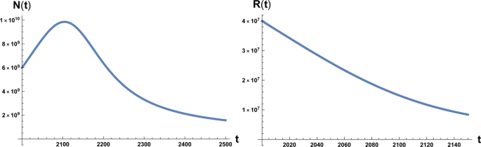
On the left: plot of the solution of Eq. (1) with the initial condition N₀ = 6 × 10⁹ at initial time t = 2000 A.C. On the right: plot of the solution of Eq. (2) with the initial condition R₀ = 4 × 10⁷. Here β = 700 and a₀ = 10⁻¹².

Full size image

Figure 2

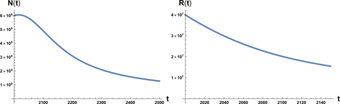
On the left: plot of the solution of Eq. (1) with the initial condition N₀ = 6 × 10⁹ at initial time t = 2000 A.C. On the right: plot of the solution of Eq. (2) with the initial condition R₀ = 4 × 10⁷. Here β = 170 and a₀ = 10⁻¹².

Full size image

Statistical model of technological development

According to Kardashev scale^7,8, in order to be able to spread through the solar system, a civilisation must be capable to build a Dyson sphere¹⁶, i.e. a maximal technological exploitation of most the energy from its local star, which in the case of the Earth with the Sun would correspond to an energy consumption of E_D ≈ 4 × 10²⁶ Watts, we call this value Dyson limit. Our actual energy consumption is estimated in E_c ≈ 10¹³ Watts (Statistical Review of World Energy source)⁹. To describe our technological evolution, we may roughly schematise the development as a dichotomous random process

where T is the level of technological development of human civilisation that we can also identify with the energy consumption. α is a constant parameter describing the technological growth rate (i.e. of T) and ξ(t) a random variable with values 0, 1. We consider therefore, based on data of global energy consumption^5,6 an exponential growth with fluctuations mainly reflecting changes in global economy. We therefore consider a modulated exponential growth process where the fluctuations in the growth rate are captured by the variable ξ(t). This variable switches between values 0, 1 with waiting times between switches distributed with density ψ(t). When ξ(t) = 0 the growth stops and resumes when ξ switches to ξ(t) = 1. If we consider T more strictly as describing the technological development, ξ(t) reflects the fact that investments in research can have interruptions as a consequence of alternation of periods of economic growth and crisis. With the following transformation,

differentiating both sides respect to t and using Eq. (5), we obtain for the transformed variable W

where (bar{xi }(t)=2[xi (t)-langle xi rangle ]) and 〈ξ〉 is the average of ξ(t) so that (bar{xi }(t)) takes the values ±1.

The above equation has been intensively studied, and a general solution for the probability distribution P(W, t) generated by a generic waiting time distribution can be found in literature¹⁷. Knowing the distribution we may evaluate the first passage time distribution in reaching the necessary level of technology to e.g. live in the extraterrestrial space or develop any other way to sustain population of the planet. This characteristic time has to be compared with the time that it will take to reach the no-return point. Knowing the first passage time distribution¹⁸ we will be able to evaluate the probability to survive for our civilisation.

If the dichotomous process is a Poissonian process with rate γ then the correlation function is an exponential, i.e.

and Eq. (7) generates for the probability density the well known telegrapher’s equation

We note that the approach that we are following is based on the assumption that at random times, exponentially distributed with rate γ, the dichotomous variable (bar{xi }) changes its value. With this assumption the solution to Eq. (9) is

where I_n(z) are the modified Bessel function of the first kind. Transforming back to the variable T we have

where for sake of compactness we set

In Laplace transform we have

The first passage time distribution, in laplace transform, is evaluated as¹⁹

Inverting the Laplace transform we obtain

which is confirmed (see Fig. 3) by numerical simulations. The time average to get the point x for the first time is given by

which interestingly is double the time it would take if a pure exponential growth occurred, depends on the ratio between final and initial value of T and is independent of γ. We also stress that this result depends on parameters directly related to the stage of development of the considered civilisation, namely the starting value T₁, that we assume to be the energy consumption E_c of the fully industrialised stage of the civilisation evolution and the final value T, that we assume to be the Dyson limit E_D, and the technological growth rate α. For the latter we may, rather optimistically, choose the value α = 0.345, following the Moore Law²⁰ (see next section). Using the data above, relative to our planet’s scenario, we obtain the estimate of 〈t〉 ≈ 180 years. From Figs. 1 and 2 we see that the estimate for the no-return time are 130 and 22 years for β = 700 and β = 170 respectively, with the latter being the most realistic value. In either case, these estimates based on average values, being less than 180 years, already portend not a favourable outcome for avoiding a catastrophic collapse. Nonetheless, in order to estimate the actual probability for avoiding collapse we cannot rely on average values, but we need to evaluate the single trajectories, and count the ones that manage to reach the Dyson limit before the ‘no-return point’. We implement this numerically as explained in the following.

Figure 3

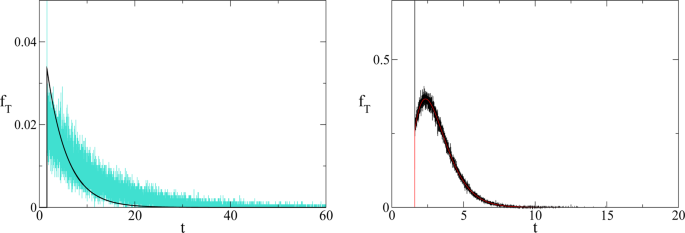
(Left) Comparison between theoretical prediction of Eq. (15) (black curve) and numerical simulation of Eq. (3) (cyan curve) for γ = 4 (arbitrary units). (Right) Comparison between theoretical prediction of Eq. (15) (red curve) and numerical simulation of Eq. (3) (black curve) for γ = 1/4 (arbitrary units).

Full size image

Figure 4

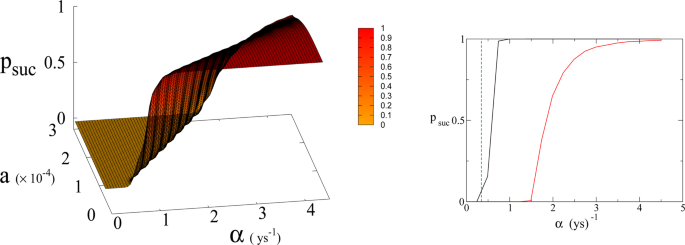
(Left panel) Probability p_suc of reaching Dyson value before reaching “no-return” point as function of α and a for β = 170. Parameter a is expressed in Km² ys⁻¹. (Right panel) 2D plot of p_suc for a = 1.5 × 10⁻⁴ Km² ys⁻¹ as a function of α. Red line is p_suc for β = 170. Black continuous lines (indistinguishable) are p_suc for β = 300 and 700 respectively (see also Fig. 6). Green dashed line indicates the value of α corresponding to Moore’s law.

Full size image

Numerical results

We run simulations of Eqs. (1), (2) and (5) simultaneously for different values of of parameters a₀ and α for fixed β and we count the number of trajectories that reach Dyson limit before the population level reaches the “no-return point” after which rapid collapse occurs. More precisely, the evolution of T is stochastic due to the dichotomous random process ξ(t), so we generate the T(t) trajectories and at the same time we follow the evolution of the population and forest density dictated by the dynamics of Eqs. (1), (2)³ until the latter dynamics reaches the no-return point (maximum in population followed by collapse). When this happens, if the trajectory in T(t) has reached the Dyson limit we count it as a success, otherwise as failure. This way we determine the probabilities and relative mean times in Figs. 5, 6 and 7. Adopting a weak sustainability point of view our model does not specify the technological mechanism by which the successful trajectories are able to find an alternative to forests and avoid collapse, we leave this undefined and link it exclusively and probabilistically to the attainment of the Dyson limit. It is important to notice that we link the technological growth process described by Eq. (5) to the economic growth and therefore we consider, for both economic and technological growth, a random sequence of growth and stagnation cycles, with mean periods of about 1 and 4 years in accordance with estimates for the driving world economy, i.e. the United States according to the National Bureau of Economic Research²¹.

Figure 5

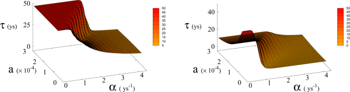
Average time τ (in years) to reach Dyson value before hitting “no-return” point (success, left) and without meeting Dyson value (failure, right) as function of α and a for β = 170. Plateau region (left panel) where τ ≥ 50 corresponds to diverging τ, i.e. Dyson value not being reached before hitting “no-return” point and therefore failure. Plateau region at τ = 0 (right panel), corresponds to failure not occurring, i.e. success. Parameter a is expressed in Km² ys⁻¹.

Full size image

Figure 6

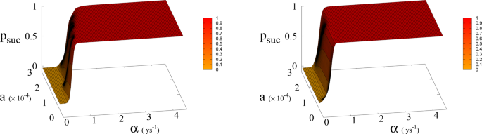
Probabilityp_suc of reaching Dyson value before hitting “no-return” point as function of α and a for β = 300 (left) and 700 (right). Parameter a is expressed in Km² ys⁻¹.

Full size image

Figure 7

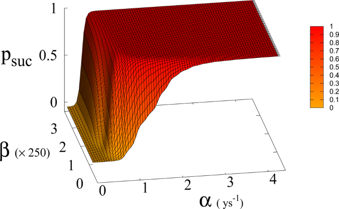
Probability of reaching Dyson value p_suc before reaching “no-return” point as function of β and α for a = 1.5 × 10⁻⁴ Km² ys⁻¹.

Full size image

In Eq. (1, 2) we redefine the variables as N′ = N/R_W and R′ = R/R_W with ({R}_{W}simeq 150times {10}^{6},K{m}^{2}) the total continental area, and replace parameter a₀ accordingly with a = a₀ × R_W = 1.5 × 10⁻⁴ Km² ys⁻¹. We run simulations accordingly starting from values ({R{prime} }_{0}) and ({N{prime} }_{0}), based respectively on the current forest surface and human population. We take values of a from 10⁻⁵ to 3 × 10⁻⁴ Km² ys⁻¹ and for α from 0.01 ys⁻¹ to 4.4 ys⁻¹. Results are shown in Figs. 4 and 6. Figure 4 shows a threshold value for the parameter α, the technological growth rate, above which there is a non-zero probability of success. This threshold value increases with the value of the other parameter a. As shown in Fig. 7 this values depends as well on the value of β and higher values of β correspond to a more favourable scenario where the transition to a non-zero probability of success occurs for smaller α, i.e. for smaller, more accessible values, of technological growth rate. More specifically, left panel of Fig. 4 shows that, for the more realistic value β = 170, a region of parameter values with non-zero probability of avoiding collapse corresponds to values of α larger than 0.5. Even assuming that the technological growth rate be comparable to the value α = log(2)/2 = 0.345 ys⁻¹, given by the Moore Law (corresponding to a doubling in size every two years), therefore, it is unlikely in this regime to avoid reaching the the catastrophic ‘no-return point’. When the realistic value of a = 1.5 × 10⁴ Km² ys⁻¹ estimated from Eq. (4), is adopted, in fact, a probability less than 10% is obtained for avoiding collapse with a Moore growth rate, even when adopting the more optimistic scenario corresponding to β = 700 (black curve in right panel of Fig. 4). While an α larger than 1.5 is needed to have a non-zero probability of avoiding collapse when β = 170 (red curve, same panel). As far as time scales are concerned, right panel of Fig. 5 shows for β = 170 that even in the range α > 0.5, corresponding to a non-zero probability of avoiding collapse, collapse is still possible, and when this occurs, the average time to the ‘no-return point’ ranges from 20 to 40 years. Left panel in same figure, shows for the same parameters, that in order to avoid catastrophe, our society has to reach the Dyson’s limit in the same average amount of time of 20–40 years.

In Fig. 7 we show the dependence of the model on the parameter β for a = 1.5 × 10⁻⁴.

Source: Ecology - nature.com