Study area
We conducted our study in the estuarine portion of the three main tributaries of Todos os Santos Bay located in Bahia state in Brazil: Paraguaçu (56,300 km2), Subaé (600 km2) and Jaguaripe (2,200 km2) Rivers29 (Fig. 2). Several anthropogenic activities, such as industrial effluents, untreated sewage, urbanization, agriculture, ports and mining activities, have decreased the environmental quality in some specific regions of our study area30. Since we were interested in analyzing the influence of environmental filters on the structure of metacommunities, each estuary studied encompassed the effect of a salinity gradient ranging from approximately 0.5 to 40 along 10 or 11 randomly chosen stations (Fig. 3). Each one of the 10 (Jaguaripe and Paraguaçu) or 11 stations (Subaé) along the salinity gradient had two randomly chosen sites. A total of 270 sites were sampled for all estuarine systems over time. In each estuary, we sampled in a gradient from the most seaward and generally deepest station (i.e., lower-numbered stations in Fig. 2) to the furthest inland and shallowest station (i.e., higher-numbered stations in Fig. 2).
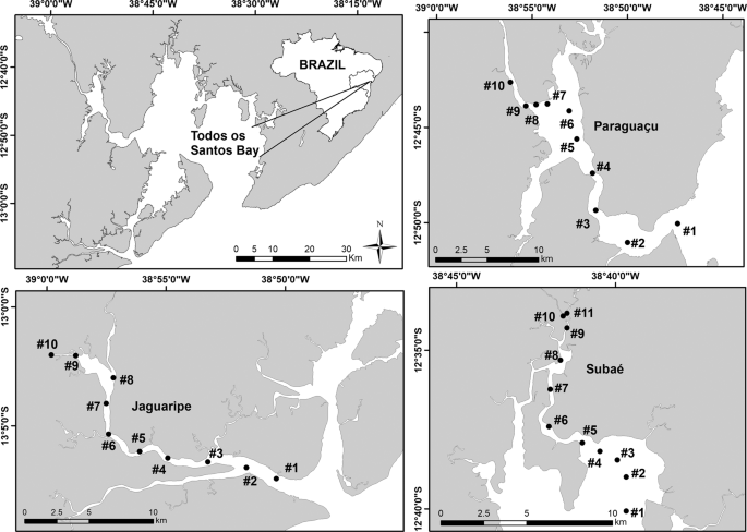
Map of the study area showing sampled stations (black dots) for each estuary (Subaé, Jaguaripe, and Paraguaçu) at Todos os Santos Bay, in Bahia, Brazil.
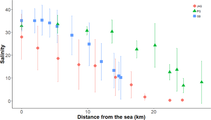
Salinity gradient from sea to freshwater in sampled sites for Jaguaripe (circles), Paraguaçu (triangles) and Subaé (squares) estuaries at Baía de Todos os Santos.
The survey took place over time in different estuaries. The Subaé estuary was sampled in five periods: Jun-2004, Mar-2006, Dec-2009, Apr-2011, and Mar-2013. The Jaguaripe estuary was sampled in four periods: May-2006, Aug-2007, Jul-2010, and Aug-2014. Finally, the Paraguaçu estuary was sampled in four periods: May and Dec-2005, Jun-2011, and Aug-2014.
Sample collection and processing
In the Paraguaçu estuary, the six replicates were collected at each station using a van Veen grab (0.05 m2, 3.2 L). In Subaé and Jaguaripe, at each station eight replicates were collected manually by divers, using corers (10 cm diameter, 0.008 m2, 1.2 L). Core sampling was not suitable in the Paraguaçu River due to the depth at some stations ( > 35 m), very strong water current and zero visibility. For both types of gear, sample infauna was collected from the water–sediment interface to a depth of 15 cm31. All macroinfaunal samples were sieved through a 0.5 mm mesh in the field, preserved in 70% alcohol and taken to the laboratory for further processing and identification. Most invertebrates were identified to family level; family has been shown to be a taxonomically sufficient descriptor of estuarine benthic invertebrates in habitats with strong gradients32 but still provide information about community identities and their temporal drift33. Also, family level was a good choice due to the scarcity of taxonomical studies of the local benthic invertebrates (with several undescribed species) and allowed comparison of the taxon distribution patterns observed in other regions21.
The environmental variables measured included salinity and sediment type (i.e., grain size). Salinity of the superficial water was measured at spring low ebb tides and recorded using a Hydrolab Data Sonde. One sediment sample was collected at each station for grain size analysis, using a 0.05 m2 van Veen grab for Paraguaçu River and a 0.008 m2 corer for Subaé and Jaguaripe. Sediment particle size was determined by standard techniques34. Salinity and each fraction of sediment grain size (i.e., pebble, gravel, very coarse sand, coarse sand, medium sand, fine sand, very fine sand and silt sand clay) were treated as environmental predictors.
Sample adequacy
In order to evaluate whether the benthic macroinfaunal family of each estuary was representatively sampled and to avoid artifactual patterns because the probability of detection of species varied, we calculated the relationship between sampling effort and family richness for each estuary for the total sampling time. The specaccum function and the species accumulation method random were used in the vegan package35 in the R environment36. Sample-based rarefaction is preferable than individual-based rarefaction to account for natural levels of sample heterogeneity in the data37.
A total of 11,328 individuals of benthic invertebrates were sampled, mainly belonging to 144 taxa of Polychaeta, Mollusca and Crustacea. Polychaeta was the most abundant phylum, followed by Mollusca and Crustacea. In spite of differences in the sampling methods (i.e., sampling gear, total area sampled, number of sites and replicates) among estuaries, most of the systems showed a near stabilization of the relationship between number of stations and richness, allowing further analyses (Supplementary Fig. 1).
Elements of metacommunity structure
We used incidence matrices (i.e., presence–absence) to estimate Elements of Metacommunity Structure (EMS). We followed the ‘range perspective’ in our analysis, which is defined by species range turnover and range boundary clumping8 as recommended38. These incidence matrices were subsequently subjected to a reciprocal averaging (also known as Correspondence Analysis, CA), an unconstrained ordination method, which positions sites having similar species composition close to each other and locating species having similar occurrence among the sites close to each other along the ordination axis39. Because we focused only on the first ordination axis, other ordination methods, such as detrended correspondence analysis, will give the same results8. When a single or at least a predominant gradient structures a community data set, the reciprocal averaging arranged matrix will display this gradient effectively.
Coherence, the first EMS metric, is based on calculating the number of embedded absences (i.e., interruptions in species distribution or in the composition of the sites) in the ordinated matrix and then comparing the empirical observed value of embedded absences (EmbAbs) to a null distribution created from simulated matrices with 1,000 iterations7,8. A large number of embedded absences (i.e., EmbAbs significantly larger than expected by chance) suggests negative coherence and leads to a checkerboard distribution of species; non-significant coherence refers to a random metacommunity type; and a small number of embedded absences (i.e., EmbAbs significantly lower than expected by chance) suggests positive coherence related to nestedness, evenly spaced, Gleasonian or Clementsian gradients8 (Fig. 1).
Turnover is evaluated if coherence is significant and positive (Fig. 1). It is measured by the number of times one species replaces another between two sites (i.e., number of replacements) in an ordinated matrix. To do this, the number of empirical replacements (turnover) was compared to the distribution of randomly generated values based on a null model distribution that randomly shifts entire ranges of species8. Significant negative turnover (i.e., replacement significantly lower than expected by chance) refers to nested subsets, while significant positive turnover (i.e., replacement significantly larger than expected by chance) refers to evenly spaced gradients (Gleasonian or Clementsian structures), requiring further analysis of boundary clumping to distinguish among them8. Furthermore, cases where coherence is significant and positive and turnover is non-significant can be regarded as quasi-structures, indicating that the effects of structuring mechanisms are weaker than in idealized structures7 (Fig. 1).
Boundary clumping is analysed using the Morisita’s Index40 and a chi-square test comparing observed and expected distributions of range boundary locations. Non-significant clumping, and values of Morisita’s index that are not different from 1, indicate randomly distributed species loss in nested subsets when turnover is negative or Gleasonian distribution when turnover is positive. Values significantly larger than 1 indicate clumped species loss in nested subsets when turnover is negative or Clementsian distribution when turnover is positive. Values significantly less than 1 indicate hyperdispersed species loss in nested subsets when turnover is negative and an evenly spaced metacommunity type when turnover is positive (Fig. 1).
The significance of coherence and turnover was tested separately using the fixed-proportional null model, where the species richness of each site was maintained (i.e., row sums were fixed), but species frequencies of occurrence (i.e., columns) were filled based on their marginal probabilities. Random matrices were produced by the r1 method using the R package vegan35 for the fixed-proportional null model, which has a more desirable combination of Type I and Type II error properties7 and has been applied successfully15,16,38,41,42. All EMS analyses were done using the metacom package43 in the R environment (version 1.5.0)36.
Nestedness
We performed ‘nestedness metric based on overlap and decreasing fill’ (NODF)44 to accurately identify nestedness along salinity gradients in estuarine benthic communities. There is some criticism about the EMS framework used to investigate idealized metacommunity patterns and especially whether the turnover test is adequate for detecting a nested pattern, as turnover and nestedness are not necessarily exclusive or opposite38,45,46. Schmera et al.46 showed that even though high turnover is frequently related to low nestedness, low turnover does not predict high nestedness. We performed NODF using the oecosimu function from the vegan package35 in the R environment (version 2.0-10)36.
Spatial predictors
We used Principal Components of Neighbour Matrices (PCNM) to generate spatial variables from geographical coordinates (e.g., latitude and longitude) represented as a Euclidean distance matrix47,48. The PCNM technique represents the spatial configuration of sample points using principal coordinates of a truncated geographic distance matrix between sampling sites. We used the resulting PCNM eigenvectors associated with the positive eigenvalues as spatial components in a global test and in a forward selection prior to variation partitioning47,49,50. PCNM analyses were done using the function pcnm in the vegan package35 in the R environment (version 2.0-10)36.
Environmental predictors
We converted environmental data to standardized Z-scores by subtracting each environmental variable from their mean and dividing by their standard deviation. The new standardized variables are thus dimensionless, with a mean of 0 and a standard deviation of 151. In addition, we tested multicollinearity using a variance inflation factor (VIF)52. When the VIF values indicated a high level of collinearity, we removed the predictor with the highest VIF value. We then recalculated VIF and repeated this process until all VIFs were below a pre-selected threshold (VIF < 3)52,53. Standardized Z-score and VIF analyses were done using the functions scale and vif.cca, respectively, in the vegan package35 in the R environment (version 2.0-10)36.
Variation partitioning
We used partial Redundancy Analysis (pRDA)51 to quantify the pure and shared contributions of environmental filters (i.e., salinity and each fraction of sediment grain size), spatial variables (i.e., variables created using PCNM) and time (i.e., sampling occasions) structuring the benthic metacommunity in the estuaries. RDA can be best understood as an extension of multiple regression that has multiple response variables (i.e., species) and a common matrix of predictors (i.e., environmental and spatial predictors)54. pRDA or variation partitioning51 may indicate the relative strength of association between each component and the metacommunity pattern of benthic macroinvertebrates. We expected environmental variables to be the main influencer of benthic metacommunity structure. In situations where environmental gradients determine most of the variation in the living community, the amount of variation in species data explained by environmental variables is fairly high55. We also included sampling period as a temporal predictor in variation partitioning because time may influence community structure, but we did not have specific expectations regarding temporal variation in benthic structures.
Prior to the pRDA, we Hellinger-transformed abundance matrices and report values based on adjusted R2 to provide unbiased estimates of explained variation and valid comparisons between sets of factors for explaining community structure54. Hellinger transformation consists of transforming the site-by-species data into relative values per site by dividing each value by the site sum, and then taking the square root of the resulting values42. It is suitable for community composition data in comparative analysis because it reduces the importance of high species abundance.
We first did a global RDA test to prevent the inflation of Type I error, and only if it was significant proceeded with forward selection using the double-stopping criterion: the usual alpha significance level (p < 0.05) and the adjusted coefficient of multiple determination (R2)49. Each eigenvector was counted as a single predictor since this approach is the most conservative in its penalization of degrees of freedom and adjusted R2 statistics50. We used forward selection to determine the environmental and spatial filters to be used in variation partitioning. Forward selection analyses for spatial and environmental predictors were done using the ordiR2step function in the vegan package35 in the R environment (version 2.0-10)36.
We carried out pRDA using the function varpart in the vegan package35 in the R environment (version 2.0-10)36. We report adjusted R2 and test the significance of the pure environmental, pure spatial and pure temporal components (P < 0.05). The total percentage of variation explained by the model (R2) is partitioned into unique and common contributions of sets of predictors54. It offers a way of dealing with the importance of spatial correlation when observations are not independent, the number of degrees of freedom in the sample is smaller than expected based on the number of observations used in the analysis, and Type I errors increase, leading to incorrect conclusions about the effect of the environment on community structure56. Statistical significance of RDA in global models was based on 999 permutations and assessed at a significance level of 0.05.
Source: Ecology - nature.com

