Exceptionally high biosphere productivity at the beginning of Marine Isotopic Stage 11

Material

The ice samples used for this study come from bag samples allocated to gas consortium (A cut) of the EPICA Dome C 2 ice core. They were stored after drilling (2002-2003) in France (Le Fontanil) at −20 °C before being transported to LSCE, Gif sur Yvette in December 2017 for analysis in first semester of 2018. In total, 53 ice samples were analysed but 3 samples were lost due to an excess of pressure in the line.

Extraction of air trapped in bubble from ice

Extraction of air trapped in bubbles of ice was performed using a semi-automatic extraction and separation line. A 5-mm-thick section of ice was removed from each sample prior to measurement to prevent any contamination from ambient air or drilling fluid. The sample is then introduced in a frozen flask (−20 °C) attached to the extraction line together with 5cc flasks of outside air (standard for isotopic composition of oxygen). For each daily sequence, two flasks of exterior air and three duplicated ice samples (i.e. 6 ice samples) were analysed. After pumping the line 40 min with samples kept at −20 °C, the ice samples are melted to extract the air trapped in the bubble from the melted ice. The air then goes through H₂O and CO₂ traps immersed in ethanol cooled at −90 °C and in liquid nitrogen (−196 °C) respectively. The gas sample is transferred in a molecular sieve at −196 °C, then in a chromatographic column (1 m*2 mm) to separate O₂ and Ar from N₂ and finally goes through another molecular sieve to purify O₂ and Ar from remaining He. The extracted air is then trapped in stainless-steel tubes in an 8 port collection manifold immerged in liquid helium (4.13 K). The method follow description from Barkan and Luz⁵⁷ except that the chromatographic column is longer (1 m instead of 20 cm) and kept at higher temperature (0 °C instead of −90 °C).

Mass spectrometer measurements

Measurements of ¹⁸O/¹⁶O, ¹⁷O/¹⁶O and ³²O₂/⁴⁰Ar (δO₂/Ar) were performed using a multi-collector mass spectrometer Thermo Scientific MAT253 run in dual inlet mode. For each extracted air sample, 3 runs of 24 dual inlet measurements were performed against a laboratory standard gas obtained by mixing commercial O₂ and commercial Ar in atmospheric concentration. The mean of the three runs were calculated for each sample and the standard mean deviation is calculated as the pooled standard deviation over all duplicate samples hence integrating the variability associated with extraction, separation and mass spectrometry analysis.

The resulting pooled standard deviations before the corrections are 0.05‰, 0.02‰, 6.4‰ and 6 per meg for δ¹⁸O_atm, δ¹⁷O_atm, δO₂/Ar measurements and Δ¹⁷O of O₂ calculation, respectively.

Atmospheric air calibration

Every day, δ¹⁸O, δ¹⁷O and δO₂/Ar of atmospheric air are measured and are then used to calibrate our measurements following:

The δ¹⁸O_{ext air} and δ¹⁷O_{ext air} were constant during the two measurement periods so that we used the average values over the two corresponding periods to correct the raw data. The daily correction was the same every day during each period.

Correction due to fractionation in the firn column

Several corrections were applied on the measured data due to fractionation in the firn. We describe here corrections due to gravitational and thermal fractionation as well as pore close-off effect.

Gravitational fractionation operates in firn due to Earth gravity field. δ¹⁸O and δ¹⁷O were obtained by corrections for this diffusive process using δ¹⁵N in neighbouring samples⁵⁸. The correction applied depends on the difference of mass between the two isotopes considered so that:

Diffusive processes operating in the firn column due to changes in temperature or because of the Earth gravity must also be taken into account. These processes lead to isotopic fractionation of O₂ that was taken into account for δ¹⁸O_atm reconstruction in the NGRIP ice core over abrupt temperature changes of the last glacial period⁵⁹. To check the effect of thermal fractionation on Δ¹⁷O of O₂, we performed measurements of Δ¹⁷O of O₂ over the top 17 m of the EastGRIP firn were a strong seasonal gradient is present. However, the resulting Δ¹⁷O of O₂ was not showing any significant deviation from the atmospheric value hence suggesting that thermal fractionation does not modify the Δ¹⁷O of O₂ of the atmosphere in the firn column (Supplementary Table 3). Moreover, in Antarctica, surface temperature variations are much lower than in Greenland during deglaciations or climatic variability of the last glacial period so that thermal fractionation is not expected to have a significant effect on the isotopic composition of trapped oxygen.

Pore close-off at the bottom of the firn has been shown to affect δO₂/N₂, δAr/N₂ with potential effects on δ¹⁵N and δ⁴⁰Ar in certain cases⁶⁰. We checked this possible effect on Δ¹⁷O of O₂ by comparing Δ¹⁷O of O₂ in bubbly ice at the top of the NEEM ice core. After correction of gravitational effect, we found a systematic enrichment of 13 per meg which could potentially bias the reconstruction of atmospheric Δ¹⁷O of O₂ from Δ¹⁷O of O₂ in trapped air.

Gas loss correction

During storage, O₂ in ice samples is subject to gas loss fractionation due to diffusion processes⁶¹ and O₂/N₂ ratio is always lower by several % in ice samples stored several years at −20 °C than ice samples stored at −50 °C⁶². Such gas loss effect is also associated with isotopic fractionation of oxygen, δ¹⁸O_atm trapped in the ice being higher when δO₂/N₂ decreases with a slope for the relationship of −0.01 (δ¹⁸O_atm vs δO₂/N₂)^17,18,63,64. We thus expect that δ¹⁷O can also be affected by this gas loss process and that it may create an anomaly of Δ¹⁷O of O₂. To check this effect, measurements of δ¹⁷O, δ¹⁸O_atm, Δ¹⁷O of O₂ and δO₂/Ar have been performed on three samples of GRIP ice core (clathrate ice stored during more than 20 years at −20 °C). Each of the three ice samples have been cut in order to analyse the interior and the exterior of the sample separately. δO₂/N₂ measurements could not be performed on exactly the same samples so that we used the δO₂/Ar measurements to estimate the amount of oxygen loss. Argon is also known to be affected by gas loss^17,61 but in a smaller extend than oxygen⁶⁵ so that the decrease of δO₂/Ar is still a good indication of larger gas loss.

Data show a systematic lower Δ¹⁷O of O₂ value in the exterior sample compared to the interior sample, paralleling the lower δO₂/Ar value in the exterior sample compared to the interior sample as expected by gas loss (Supplementary Table 1). This systematic relationship and the Δ¹⁷O of O₂ and δO₂/Ar values can be used to propose a correction for the Δ¹⁷O of O₂ that takes into account the gas loss effect:

Comparison of EDC Δ¹⁷O of O₂ with previous Δ¹⁷O of O₂ record

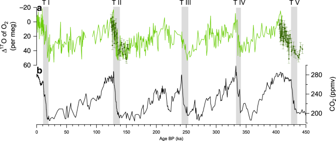
Previous Δ¹⁷O of O₂ measurements only took into account correction linked with gravitational fractionation. As a consequence, we checked the consistency of previous records performed on the GISP2 and Vostok ice core with our new EDC data by measuring again Δ¹⁷O of O₂ over Termination II using EDC samples and integrating the aforementioned correction (Fig. 1).

Flux of oxygen associated with biosphere productivity

We follow here the calculation of the flux of oxygen associated with biosphere productivity described in Landais et al.³³.

Since the atmospheric Δ¹⁷O of O₂ (Δ¹⁷O_atm) is influenced by the exchanges with biosphere and stratosphere, it is possible to write the following equation in a 3-box system at equilibrium (biosphere—bio-, atmosphere—atm-, stratosphere—strat-):

where F_bio is the flux of oxygen exchanged by photosynthesis and respiration (both fluxes being considered at equilibrium) and F_strat is the flux of oxygen exchanged between the lower atmosphere (or troposphere) and the stratosphere (fluxes in and out of the stratosphere are assumed equal).

To reconstruct past biospheric fluxes between terrestrial/oceanic biosphere and atmosphere based on Δ¹⁷O of O₂, it is necessary to know the evolution of the stratospheric flux as well as of the Δ¹⁷O_strat. Luz et al.²⁰ and Blunier et al.²² showed that a good assumption is to consider that the production rate of depleted O₂ in the stratosphere can be related to the atmospheric CO₂ concentration. It is then possible to express the evolution of biosphere oxygen flux in the past compared to pre-industrial from the following equation:

where F_bio,t is the biosphere oxygen flux at a given time, F_{bio,pre-industrial} is the present time biosphere oxygen flux, (CO₂)_t and (CO₂)_{pre-industrial} correspond to the atmospheric CO₂ concentration at a given time and at the pre-industrial period respectively, Δ¹⁷O_{bio,pre-industrial} and Δ¹⁷O_bio,t are the values of Δ¹⁷O of O₂ in an atmosphere that would only be influenced by exchanges with the biosphere at the present time and at a given time respectively. Δ¹⁷O_{atm, t} is the Δ¹⁷O of O₂ of the atmosphere at a given time measured in the air trapped in ice core. We refer to pre-industrial period because of the long residence time of oxygen in the atmosphere (>1000 years), Δ¹⁷O of O₂ is not exhibiting any significant variation over the last centuries.

Δ¹⁷O_bio can be calculated from the fractionation coefficients associated with the different processes leading to oxygen fluxes in the biosphere (mainly photosynthesis, dark respiration and photorespiration). Detailed calculations of Δ¹⁷O_bio at the LGM and pre-industrial periods were obtained in Landais et al.³³ taking into account uncertainties in the determination of the fractionation coefficients³⁴ as well as on the relative fluxes of oxygen (Supplementary Table 2).

From the calculation of Δ¹⁷O_{bio, pre-industrial} and Δ¹⁷O_bio,LGM (Supplementary Table 2), Δ¹⁷O_bio,t is calculated through a scaling on the variations of CO₂ concentration between pre-industrial period (280 ppmv) and the LGM (190 ppmv)⁶⁶ such as

Details on uncertainty in photosynthesis fractionation

We performed sensitivity tests to compare biosphere productivity reconstructions without any fractionation and reconstruction with the different fractionation effects during marine photosynthesis as observed in Eisenstadt et al.³⁷. The largest change on the reconstructed biosphere productivity is obtained using the observed photosynthesis fractionation effect associated with Emiliania huxleyi (δ¹⁸O = 5.81‰ and slope between ln(δ¹⁷O + 1) and ln(δ¹⁸O + 1) of 0.5253). The reconstructed global biosphere productivity is lower with such fractionation effect: the MIS 11 productivity level is decreased by 3% with such fractionation effect compared to the reconstruction with no fractionation at photosynthesis (i.e. the average situation, see Supplementary Table 2).

Details on uncertainty in respiration fractionation

When taking into account the maximum effect, i.e. a decrease of 0.005 for the slope of the relationship between ln(δ¹⁷O + 1) and ln(δ¹⁸O + 1) during respiration, we end up with a decrease of Δ¹⁷O_bio by 65 ppm. The resulting biosphere productivity reconstruction is about 16% higher during MIS 11 than the average situation (Supplementary Table 2) leading to an anomalously high O₂ flux associated with gross primary productivity during Termination V.

Validation of the biosphere productivity reconstruction

The three sensitivity tests displayed (uncertainty on photosynthesis fractionation, on respiration fractionation and on fractionation within the water cycle) suggest that the biosphere productivity during MIS 11 is significantly higher than for our current interglacial, leading to the envelop displayed on Supplementary Fig. 2. Actually, explaining the Δ¹⁷O of O₂ anomaly without invoking a significant increase of the global productivity at the beginning of MIS 11 requires huge change of the Δ¹⁷O of O₂ produced by terrestrial biosphere (through changes in fractionation factor or changes in water cycle, hypothesis 1) or of the ratio of oceanic to terrestrial biosphere productivity (hypothesis 2). These two possibilities are rather unrealistic as detailed below.

In hypothesis 1, an increase of 30 ppm for Δ ¹⁷O of O₂ produced by terrestrial biosphere is needed. This can be obtained either by a huge change in the fractionation factors between our current interglacial and MIS 11 (which is not realistic since these are based on physical processes which do not vary with time) or by a change of water cycle during MIS 11 with respect to present-day value. To reach this 30 ppm increase through modification of the water cycle, one option is to increase the ¹⁷O-excess of meteoric water by 30 ppm during MIS 11 compared to our current interglacial. We do not have ¹⁷O-excess values for MIS 11 yet, but ice core ¹⁷O-excess values obtained for the last interglacial are very similar to values obtained for the present interglacial³⁹. Moreover, increasing ¹⁷O-excess by 30 ppm would require unrealistic decrease of relative humidity at evaporation (by 30%, Barkan and Luz⁶⁷) during MIS 11 compared to our present interglacial. Finally, an increase of the mean δ¹⁸O and δ¹⁷O of meteoric water used by the plant along the meteoric water line (i.e. without global change in the global ¹⁷O-excess) would as well be a solution (see Fig. 4 of Landais et al.³³) but to reach the expected increase of 30 ppm in Δ ¹⁷O of O₂ produced by the terrestrial biosphere, it would require an increase of global mean δ¹⁸O of meteoric water by ~3 ‰ with respect to present-day that will be transmitted to the global δ¹⁸O_atm. The δ¹⁸O_atm during MIS 11 is between 0 and 0.5 ‰ higher than during MIS 1 so that it does not support this hypothesis.

Hypothesis 2 requires an increase of the oceanic vs terrestrial productivity by a factor of 2 during MIS 11 compared to present-day value. This does not go along available observations suggesting an increase in the ratio of terrestrial to oceanic productivity during MIS 11 (see main text) and is still well above the uncertainty for the variation of the ratio of oceanic to terrestrial productivity during our interglacial period (14%, Supplementary Table 2).

An additional validation of our reconstruction of exceptional productivity during the beginning of MIS 11 comes from the comparison of our reconstruction with the oxygen biosphere productivity variations obtained by Blunier et al.²² over the last four terminations using a different vegetation model and different formulation of the link between atmospheric CO₂ and flux of Δ¹⁷O of O₂ anomaly from the stratosphere. Indeed, in our approach, we directly dealt with Δ¹⁷O of O₂ anomaly in the box model while it may be more appropriate to deal with the δ¹⁷O and δ¹⁸O of O₂ values as done in Blunier et al.²² and suggested by Prokopenko et al.⁶⁸. We thus compared our reconstruction with the one performed with the model of Blunier et al.²² (Supplementary Fig. 2). The smaller difference in the oxygen flux associated with oxygen productivity between glacial and interglacial periods in Blunier et al.²² mainly comes from the different formulations of the dependency of the stratospheric anomaly Δ¹⁷O of O₂ to CO₂ atmospheric concentration. Another difference comes from the variations in the triple isotopic composition of oxygen in water between glacial and interglacial periods not taken into account in Landais et al.³³. We took this possible variation into account in our approach through the third sensitivity test explained above. We ran here the model of Blunier et al.²² over the new Termination V data. The comparison between the two methods of reconstruction (Landais et al.³³ vs Blunier et al.²²) is significant. The biosphere productivity increase at the end of Termination V is less important using the Blunier et al.²² approach than using the Landais et al.³³: 10% larger than for other interglacial periods following Blunier et al.²² instead of 20% on average following Landais et al.³³. Still, both approaches show that the biosphere productivity increase over Termination V is exceptional compared to the younger terminations.

Source: Ecology - nature.com