Excess sulfur and Fe elements drive changes in soil and vegetation at abandoned coal gangues, Guizhou China

Study area

The research was conducted in Huaxi District (106°27′–106°52E, 26°11′–26°34′) in the middle of Guizhou province. Huaxi District is located on the eastern slope of the Yunnan–Guizhou Plateau and has a subtropical monsoon humid climate, though it is also affected by its high altitude (the average altitude is 999 m), being cool in summer and warm in winter. The vertical decline rate of high temperatures is 0.6 °C/100 m in summer and only 0.4 °C/100 m in winter. The average annual temperature in the region is 14.9 °C, with 23.3 °C as the average highest temperature in July, and 4.7 °C as the average lowest temperature in January. The average number of days in January below 0 °C is 10.5 days, and the average number of days in July above 30 °C is 5.5 days. The average precipitation is abundant, 1,178.1 mm. July has the most precipitation. Huaxi district tends to have 75 days of spring, 89 days of summer, 68 days of autumn, and 133 days of winter, based on the average daily temperature (> 20 °C is summer, 10–20 °C s spring, 20–10 °C in autumn, and < 10 °C is winter). The annual frost-free period lasts 285 days. The average annual relative humidity is 81%. The average annual sunshine duration is 1,274.2 h, and the relative sunshine duration is 29%³⁴.

The soil in the study area is zonal yellow soil, which is influenced by geological structure and lithology. The main agrotypes are yellow soil, lime soil and purple soil. The study area was located in a typical subtropical long-green broad-leaved forest vegetation belt, but the original vegetation has mostly disappeared, leaving behind only some typical tree species, such as Viburnum henryi, Cinnamomum bodinieri, etc. Introduced vegetation is mainly composed of Chinese fir and Pinus massoniana Lamb. plantations. The forest coverage rate of the whole region is at 48.38%. The study area is home to more than 120 families of plants and more than 1,000 species, including rare trees such as Emmenopterys henryi, Hemlock, Zelkova schneideriana, Keteleeria fortunei and so on.

The mineral resources in the area are mainly former coal mines, with proven existing reserves of 310 million tons and recoverable reserves of 110 million tons. Before 2011, coal mines were widely distributed throughout the district and the coal gangue they produced was piled up outside each. With the strengthened environmental protection efforts after 2011, most of the coal mines were closed, but the coal gangue remains.

Field sampling

The three different selected coal mines (GP 1, 2 and 3) produced the same annual output of 90,000 tons in their average operational year. The coal gangue was stacked along the slope of the coal hole at each site. The area where the acid mine drainage possibly flowed from the abandoned mine was excluded from the selected plots. Above, in the center of and below these gangue dumps at each abandoned mine, a 2 m × 2 m plot was demarcated for vegetative investigation and sampling. Species, plant height, percent coverage and plant numbers were surveyed and recorded. Coal gangue and soil samples were collected (0–20 cm) using a soil auger (10 cm) with the five-point sampling method. Litter covering the sites was removed before sampling. Then, the five samples from the 2 m × 2 m plots were mixed into one sample for each plot. To homogenize the soil material, the samples were passed through a 2-mm sieve, which also removed live roots, mycorrhizal mycelia and coarse plant remnants. The soil samples were taken to the laboratory and divided into three subsamples. The subsamples for chemical analysis were air dried through a 0.15 mm sieve and stored at room temperature for the chemical analyses, and the subsamples for pH were passed through a 2-mm sieve.

In contrast, three plots 100 m away from each gangue were selected as control areas (CK-near). The same plot plant survey and soil sample collection methods were conducted in the CK-near plots. Finally, an additional control group was surveyed to represent unmined land in a natural state. Four control plots (CK-far) of forest, farmland and lakeside that were distant from any coal mine were chosen, and then the 2 m × 2 m plot vegetation surveys and soil sampling were conducted there too (Table 3 and Fig. 4).

Figure 4

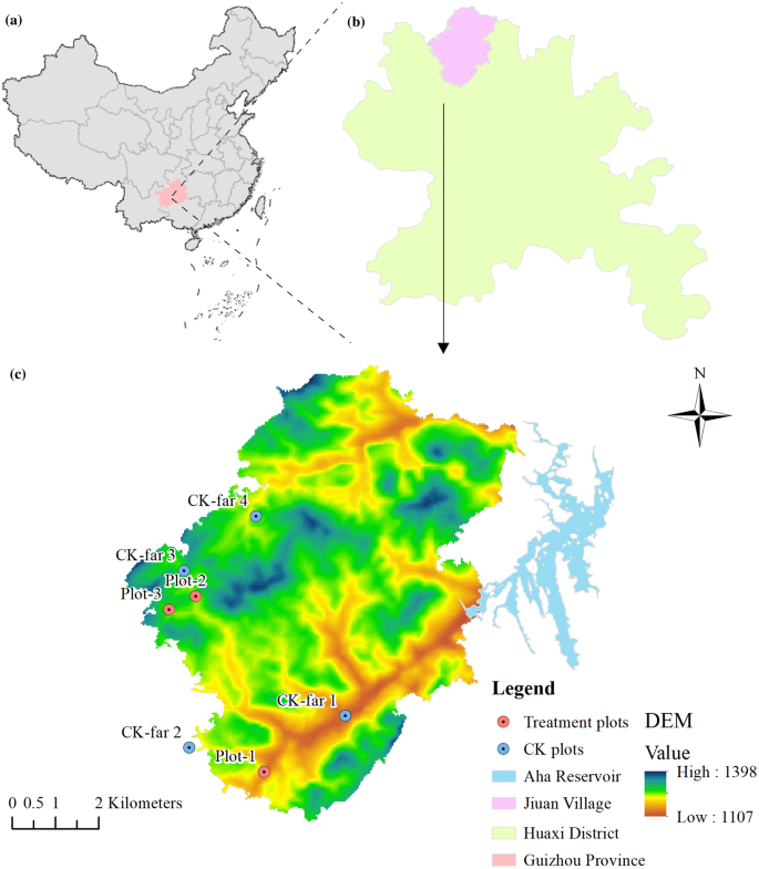
The geographical location information of the study area and distribution of sampling sites (ArcGIS Desktop. 10.3. ESRI, California, US. https://desktop.arcgis.com).

Full size image

Laboratory analysis

The levels of heavy metals (Cd, Cr, Cu, Ni, Zn, Mn, Pb) and As in the soil was tested using the national standard of China (HJ803-2016)³⁵, where all samples are acid digested following a two-step digestion method that helps retain volatile elements. This consists of a “aqua regia” extraction followed by acid digestion of the residue. The resulting solution was then analyzed using an inductively coupled plasma mass spectrometer (ICP-MS, 7500a; Agilent China) for major and selected trace elements.

Iron levels in soil were determined using the national standard also (HJ 804-2016)³⁵: the soil samples were air-dried, grinded and sifted to 2 mm. 10.0 g samples (accurate to 0.01 g) were placed in a 100 mL triangular bottle and 20.0 mL extract liquid (c (TEA) = 0.1 mol/L, c (CaCl₂) = 0.01 mol/L, c (DTPA) = 0.005mol /L); pH = 7.3) was added. Then it was shaken at 20 °C ± 2 °C at a speed of 160–200 r/min for 2 h. The extraction solution was then slowly poured into the centrifuge tube and centrifuged for 10 min. The supernatant was isolated within 48 h after gravity filtration using medium-speed quantitative filter paper. A blank control supernatant was also made at the same time.

Hg levels in soil were determined using the national standard (GB/T 17136-1997): 0.5 g soil samples were wetted with a small amount of distilled water in a 150 mL volumetric flask. Then 10 mL of HNO₃ and H₂SO₄ solution were added (1:1). After the intense reactions stopped, 10 mL of distilled water were added, and then 10 mL 0.02 g/mL K₂MnSO₄ solution. An electric heating plate was used to slowly heat the solution to near boiling, and this state was maintained for 30–60 min, being sure to add K₂MnSO₄ solution when the purple dissipated to ensure that K₂MnSO₄ was still present. Then the solution was cooled by shaking while adding 0.2 g/mL of hydroxylamine hydrochloride solution until the purple color of K₂MnSO₄ faded. And then tested with a cold atomic absorption mercury meter (F732-V; Hua Guang, Shanghai).

The soil sulfur concentrations were measured directly from a subset of air-dried samples using an elemental analyzer (Thermo Scientific FLASH 2000 CHNS/O; Waltham, MA, USA).

The soil pH values were determined using the standard method (HJ 962-2018), so the soil samples were air-dried, grinded and sifted to 2 mm, and then tested with a pH meter (Sartorius PB-10).

Determination of cation exchange capacity in soils were determined using the standard procedure (LY/T 1243-1999) with a centrifuge (TG-16W; Jinan Xinbei, China).

Data analysis

The plant biodiversity indices were calculated as follows:

Shannon–Wiener index:

Pielou index:

Important value:

Ni: the important value of species i; N: the sum of the important values of all species in the plots; S: the number of species in the plot.

SPSS 20.0 (IBM, Chicago, USA) and R³⁶ were used for all statistical analyses. ArcGIS 10.3 was used to make the distribution of sampling sites. Each plot was considered an experimental unit, and the replicated data was averaged among the plot types prior to analysis. Prior to performing ANOVA, all variables were checked for normality (Kolmogorov Smirnov test) and homogeneity (Levene’s test). Then ANOVA analysis was performed. All results are reported as the mean value ± standard error. We considered p < 0.05 to be statistically significant. To examine the relationship between soil chemical variables, data from 22 independent plots was pooled and Pearson relationships were examined using the “Performance Analytics” package in R.

Source: Ecology - nature.com