Global patterns of multi-model ensemble animal biomass
To evaluate present-day patterns of marine animal biomass, we calculated the multi-model ensemble mean biomass within each grid cell between 2006 and 2016 in standardized units of percentage of the global maximum (%; Fig. 2a). Peak biomass levels emerged in most upwelling regions, and at high temperate latitudes (~50–60°N and °S). The lowest animal biomass concentrations were observed at lower latitudes (<30°N and °S), particularly in the oligotrophic gyres. Average biomass was positively related to latitudinal gradients in average net primary production (NPP) and negatively related to gradients in sea surface temperature (SST), especially between ~50°N and °S, but less so at higher latitudes (Fig. 2a). Here, the prevalence of diatoms was often elevated, potentially increasing the fraction of NPP transferred to consumers rather than to the microbial loop, leading to higher animal biomass than would be expected from NPP or SST alone4. A linear regression model containing all three variables explained substantially more of the spatial variation in animal biomass (78%) than did any single variable (17–51%). These findings suggest that observed biomass patterns are explained by both biogeochemical (SST and NPP) and ecological variables (species composition) and highlight the importance of accurately incorporating microbial food chain dynamics and size-based predation35 as do most of the MEMs used here3. As we omitted cells containing <3 projections, biomass patterns could not be examined in many nearshore locations.
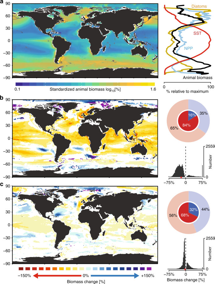
a Average standardized biomass of marine animals from multi-model projections for the contemporary period (2006–2016). Left: Map depicts animal biomass density in each grid cell, relative to the global maximum and normalized. Gray lines depict the 200 m isobath. Right: graph shows the latitudinal variation in present-day animal biomass (black), SST (red), NPP (blue), and diatom frequency (yellow). b, c Maps of projected future change in animal biomass between 2006 and 2100, relative to the reference period (2006–2016) under a worst-case scenario RCP8.5 (b) and strong mitigation scenario RCP2.6 (c). White depicts grid cells containing non-significant trends (p > 0.05) or containing insufficient data for analysis. Circular histograms depict the proportion of grid cells where analyses were possible that contained increasing (blue) or declining (red) changes. Inner opaque shading depicts changes that were statistically significant (p < 0.05), and outer shading depicts those that were both statistically significant and non-significant. Histograms show the distribution of all statistically significant predicted changes per grid cell with global means denoted as red arrows. Projected changes in b, c were estimated using longitudinal models. Data sources are listed in Table 1.
Projected future changes in marine animal biomass
Climate change scenarios had a large effect on projected biomass trends. Under a worst-case scenario (RCP8.5, Fig. 2b), 84% of statistically significant trends (p < 0.05) projected a decline in animal biomass over the 21st century, with a global median change of −22%. Rapid biomass declines were projected across most ocean areas (60°S to 60°N) but were particularly pronounced in the North Atlantic Ocean. Under a strong mitigation scenario (RCP2.6, Fig. 2c), 68% of significant trends exhibited declining biomass, with a global median change of −4.8%. Despite the overall prevalence of negative trends, some large biomass increases (>75%) were projected, particularly in the high Arctic Oceans.
Our analysis suggests that statistically significant biomass changes between 2006 and 2100 will occur in 40% (RCP2.6) or 57% (RCP8.5) of the global ocean, respectively (Fig. 2b, c). For the remaining cells, the signal of biomass change was not separable from the background variability. The estimates of biomass change and their uncertainty were different from those obtained using multi-model ensemble averaging (see Supplementary Methods for details). When present, differences between longitudinal vs. MMEA trends tended to be large and driven by trends identified by the longitudinal models as non-significant. By using longitudinal models, these highly uncertain estimates can be identified and removed (Fig. 2b, c), or statistically accounted for in subsequent analyses.
Relating future biomass changes to SES
To explore the consequences of projected biomass changes within a broader ecological and societal context, we related them to present-day geographical patterns of fisheries productivity, human stressors and indicators of SES. Indicators of fisheries productivity included annual reported and estimated commercial fishery landings, as well as illegal and unreported fishing activity (Table 1, Supplementary Table 1). Stressors included both multivariate indices of cumulative human impacts36, as well as individual stressors such as pollution, for example. SES indicators assessed development and nutritional status, social condition, ecological health, and climate change vulnerability of 106 maritime states (see Methods section, Table 1, and Supplementary Table 1 for a complete list of indicators). The SES indicators were split into those for which higher scores denoted improved condition (states), and those where increasing scores indicated reduced condition (pressures). Except for officially reported FAO fishery landings, which are made available at the scale of FAO statistical areas (n = 18), all spatial relationships between projected biomass changes and fisheries and human stressors were tested at the scale of marine ecoregions37, while SES indicators were examined at the scale of individual states’ exclusive economic zones (EEZs).
Under a worst-case emission scenario (RCP8.5), consistent negative relationships emerged between projected animal biomass change and fisheries productivity: greater biomass declines were projected for areas that currently support higher fishery yields (Fig. 3a, d). This implies that fisheries yield may decline disproportionally in more productive fishing grounds. This relationship was observed using two separate sources of landings data (Fig. 3d; ref. 38), suggesting that it is robust across data sources and spatial scales. The Northeast Atlantic is a notable outlier to this global relationship, as it supports the second-largest fishery landings by area but is projected to experience relatively small biomass losses when averaged spatially (Fig. 3a). The apparent higher resistance of Northeast Atlantic marine ecosystems to climate effects is hypothesized to be related to elevated ocean temperatures and species diversity there, relative to the Northwest Atlantic39,40, which can promote stability41. The Arctic is another outlier, supporting virtually no fishery landings at present, but projected to experience the greatest animal biomass increases (>30%) over the next century under RCP8.5 (Fig. 3a).
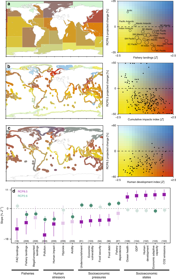
a–c Bivariate relationships between the projected animal biomass changes under a worst-case emission scenario (RCP8.5) and a total fisheries landings within 18 FAO statistical areas, b average cumulative human impacts within marine ecoregions, and c the human development index of maritime states. Bivariate maps (left panels) depict the spatial distribution of the relationships shown in the right panels. Dark and light blue depict projected biomass increase, red, orange, and yellow depict decline; horizontal line denotes no change in biomass. Symbol size in (a) depicts the geographic size of the FAO areas. d Estimated slopes from relationships between spatial gradients in 17 indicators of fisheries productivity, human stressors, and socioeconomic status (see methods for details) and projected biomass changes. Green circles are biomass changes under RCP2.6 and purple squares under RCP8.5; lines depict the 95% CIs. Darker, opaque points denote statistically significant interactions (p < 0.05), and lighter, semi-transparent points are non-significant. The sample sizes of the relationships are in parentheses. Negative slopes indicate stronger biomass declines in locations where indicators are largest and vice versa. All indicators in a–d have been standardized to units of variance from the mean.
Understanding future redistributions of fisheries biomass may be useful in anticipating and mitigating potential conflicts over fish and related social systems1. For instance, a northward shift in the distribution of Atlantic mackerel after 2007 instigated a conflict over fishing quotas between the European Union (EU), Norway, Iceland and the Faroe Islands, eroding the sustainability of the fishery42. The response of fisheries to projected redistributions of biomass will depend on additional factors such as profitability of fishing in potentially remote locations, which may be less accessible, the location of marine protected areas, and species-specific responses to climate change and other stressors.
Under RCP8.5, significant negative relationships were also found between the spatial distribution of biomass change and both cumulative (Fig. 3b) and individual (Fig. 3d) human stressors. This result suggests that the greatest climate-driven biomass losses will occur in locations that presently experience multiple additional human stressors, most of which are not accounted for by the MEMs used here3. Therefore, the biomass changes that we describe may be conservative estimates, as there will be additional impacts from fishing, bycatch, pollution, and other human impacts, which could make ecological communities more susceptible to the effects of climate change. These interactions were much weaker under the strong mitigation scenario (RCP2.6) but remained statistically significant for several indicators (green points in Fig. 3d).
Furthermore, under RCP8.5, consistent relationships were also observed between projected animal biomass changes and SES indicators (Fig. 3c, d), with more severe declines projected in regions with low SES. For example, Fig. 3c shows geographic patterns of projected biomass change and the human development index (HDI) within each EEZ (Fig. 3c, map), as well as the emergent relationship between them (Fig. 3c, right panel). The significant positive relationship between the HDI (Fig. 3c) and the mean rate of projected biomass change under RCP8.5 (p < 0.0001; r2 = 0.16) indicates that higher climate-driven biomass losses are projected to disproportionally occur within the EEZs of the least developed states. In addition to development status, states experiencing the greatest pressures such as high levels of undernourishment, food debt and insecurity, fishery dependency, and economic vulnerability to climate change are projected to experience the greatest losses of marine animal biomass over the coming century. These states also have the lowest ocean health scores, lowest wealth and adaptive capacity, and contribute the least to global CO2 emissions on a per capita (r2 = 0.13; p < 0.0001) and national basis (r2 = 0.1; p < 0.0001). The relationships between projected biomass and almost all SES indicators became weaker and often non-significant under a strong greenhouse gas mitigation scenario (RCP2.6; Fig. 3d).
Under RCP8.5, states that currently have a higher proportion of undernourishment are projected to experience the largest climate-driven reductions in animal biomass. This relationship is troubling, given that seafood accounts for 14–17% of the global animal protein consumed by humans, but with much higher reliance in small island states, where it is vital to maintaining good nutrition and health43. Declining animal biomass within the EEZs of states that are already experiencing poor nutrition may further exacerbate these deficiencies, particularly as these states also tend to be more dependent on fisheries, have low food security and high food debts (Fig. 3d). Changes in nutrition related to declining fisheries productivity could potentially be offset by increased agricultural production, aquaculture, or modifying food distribution systems12. Yet, recent studies have also highlighted the importance of seafood as a critical source of essential micronutrients that are currently lacking in the diets of up to 2 billion people44. These micronutrient deficiencies and their consequences are particularly severe in Asian and African countries45,46, many of which are projected to experience severe reductions in marine animal biomass under RCP8.5 (Fig. 2b).
Effects of emission mitigation on animal biomass projections
To explicitly evaluate the effect of strong emission mitigation on future animal biomass, we calculated the difference in projected biomass with the strongest mitigation scenario (RCP2.6) relative to those under a worst-case scenario (RCP8.5) within each EEZ and by continent (Fig. 4). The relationship between projected biomass under RCPs 8.5 and 2.6 was positive (r = 0.53) but also suggested that the effects of strong mitigation on biomass were not purely additive: some states experienced disproportionate biomass gains (Fig. 4a, above diagonal line) or losses (Fig. 4a, below diagonal line) from strong, relative to weak mitigation. Although mitigation led to increased biomass relative to worst-case emissions within the EEZs of almost all states, it resulted in declines within the EEZs of Morocco (−1%), Chile (−10%), Spain (−12%), and Russia (−12%; Fig. 4a). Relative to a worst-case scenario, the largest biomass gains from mitigation were observed for African, Asian, and South American states, including Yemen (50%), Oman (49%), Cambodia (48%), Guinea Bissau (46%), Suriname (45%), and Pakistan (44%).
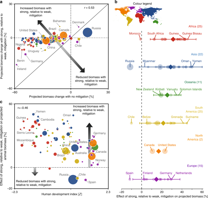
a Relationship between average projected animal biomass change across EEZs under a worst-case (RCP8.5) vs. strong mitigation scenario (RCP2.6). Horizontal and vertical dashed lines denote no change in projected biomass. The solid line represents a 1:1 relationship; points above this line depict EEZs in which strong (RCP2.6), relative to weak (RCP8.5), mitigation leads to greater biomass and vice versa. b Change in projected animal biomass resulting from strong, relative to weak mitigation within maritime EEZs (semitransparent circles) summarized within major continents (colors). The mean effect of emission mitigation on animal biomass for each continent is shown as opaque symbols with lines denoting the 95% CIs where n > 3. The number of EEZs is in parentheses. Points to the right of the vertical line denote biomass increases with strong emission mitigation relative to the worst-case scenario. c Effect of strong, relative to weak, mitigation on projected animal biomass within EEZs in relation to development status. Points above the horizontal line depict increased animal biomass with strong, relative to weak, mitigation and vice versa. For a–c, symbol size depicts the size of the EEZs and colors the continent; orange = North America, yellow = South America, purple = Europe, red = Africa, blue = Asia, and green = Oceania.
On a regional basis, the largest average biomass increases due to strong, relative to weak, greenhouse gas mitigation were projected for states in Africa, Asia, Oceania, and South America, with European and North American states experiencing lower relative biomass gains (Fig. 4b). Although the average effects of mitigation were spatially variable, significant effects were apparent within Africa and Oceania. These continental-scale effects suggested that the benefits of strong relative to weak mitigation, here denoted as biomass increases, will be most experienced by states within lesser developed regions. This hypothesis was supported by examining the effect of strong relative to weak mitigation on animal biomass along gradients in the human development index (HDI; Fig. 4c). A negative correlation was found between mitigation benefits and HDI (r = −0.46; p < 0.0001), indicating substantial benefits of strong, relative to weak mitigation for the least developed states and vice versa.
Source: Ecology - nature.com
