Current and past distribution ranges
We used species range maps from the 1970s24 and the present day, following IUCN Red List taxonomy, to measure the past change in species’ distributions. We represented the current distribution of terrestrial mammal species using the most recent maps of geographical ranges from the IUCN Red List of Threatened Species6, excluding all human-mediated introductions, and the reintroductions that occurred after 1970. Similar to current IUCN distribution ranges, all the maps we collected for the 1970s are expert-based. We included in the analysis only those species’ maps produced following mapping protocols reflecting current IUCN Red List standards6, and for which the 1970s distribution was compatible with textual descriptions of the past range in the recent literature24. Distribution ranges were available from the literature as polygons, with the exception of Australian maps, for which we extrapolated occurrence records from range maps in the last action plan of Australian mammals9. This action plan contains distributional data that the experts collated from individual datasets maintained by museums and government conservation agencies of all Australian states and territories. For each of the 204 mammal species, a polygonal map of the range was created using all distributional information available, along with knowledge of habitat, elevation limits and other expert knowledge of the taxon, following IUCN6. These polygons display the limits of each species’ distribution. For non-Australian species, maps have been revised by a certified IUCN Red List Assessor, M.P., and the Coordinator of the Global Mammal Assessment for IUCN, C.R. Australian mammals have been revised by A.A.B. and J.C.Z.W., members of the IUCN Species Survival Commission (SSC) Australian Marsupials and Monotremes Specialist Group, responsible for the IUCN Red List assessments of Australian mammals, and lead authors of the Australian mammals action plan. We looked at literature evidence to support changes observed between past and present ranges, to make sure that any difference in distribution derived from a real change, and was not an artefact of improved knowledge. In order to avoid uncertainty related to improved information on species’ distribution, we disregarded non-genuine changes in Red List status associated with changes in species’ ranges. For example, the 1970s maps of Herpestes sanguineus we found in the literature included most of Sub-Saharan Africa, with the exception of southern Africa and Western Namibia. However, it seems that the species today is only patchy distributed in Gabon, marginally in Congo, South Africa and Equatorial Guinea, and lost vast portions of its range in Cameroon, Democratic Republic of Congo, Nigeria and Central African Republic50, but we could not find enough evidence in the literature to support these reductions. Hence, we decided to exclude this species and many others with similar uncertainties from the database. Another example of species excluded from our data is Sus cebifrons. This species is endemic to the West Visayan Islands in the Philippines. The species is currently classified as Critically Endangered and declining51, but its range in Panay, the island with the largest population, is bigger than the one we found for the 1970s. Since it is not realistic, we decided to exclude the species from the analysis. We georeferenced and digitised all the maps with QGIS v3.2 to create vector data.
We obtained past distribution ranges for a total of 204 species. Although this sample represents only about 5% of all terrestrial non-volant mammals, it includes representatives of all major taxonomic orders and all terrestrial realms (Supplementary Table 1). In addition, we checked for inclusion of extreme values in the life-history predictors by comparing the probability-density functions of body mass and weaning age (the traits with the highest predictive importance in our models) in our sample and in all terrestrial non-volant mammals (Supplementary Fig. 9).
Distribution range comparison
In order to measure the maximum possible range expansion of the species in the study period, we created a buffer around the past range of each species, depicting the area that the species could theoretically colonise through dispersal during the study period (Supplementary Fig. 1)
$${mathrm{BR}} = D * left( {{it{Delta}} t/{mathrm{AFR}}} right),$$
(1)
where BR is the buffer radius (in km), D is the species dispersal capacity (in km), Δt is the time interval of the study period (in years) and AFR is the species age at first reproduction (in years). Dispersal values were calculated with the formula provided by Santini et al.30, and age at first reproduction estimates was mainly obtained from PanTHERIA52 and AnAge53 database, following the methods used in Pacifici et al.54 This allowed us to quantify how much of the potential range expansion—within the buffer around past distribution range—was realised by each species. By using age at first reproduction, there was no species whose current range went beyond the potential colonisation buffer around the past range. To be more conservative in terms of species’ potential colonisation, we also performed a sensitivity analysis by using generation-length estimates (from Pacifici et al.54) instead of age at first reproduction. This approach represents a more conservative colonisation scenario where members of one of the litters produced by an individual during its reproductive lifespan will disperse in a given direction, and members of one of their litters will do the same. In repeating our analyses under both scenarios, we showed that our results are robust to uncertainty associated with estimates of species’ colonisation potential. We measured range expansion as the percentage of area gained within the buffer area (Supplementary Data 1). This allowed to measure, for each species, the condition of habitats in areas that could be potentially reached by the species.
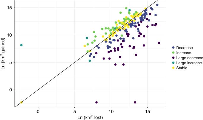
Range contraction was computed by calculating the percentage of area lost with respect to the past range (Supplementary Data 1). In order to identify proportional change in range size, we also computed the percentage of area gained with respect to the past range (Supplementary Data 1). Our approach allowed us to include the same set of species, both in the range contraction and in the range expansion model, quantifying extrinsic variables within the past range and the potential expansion buffer for all species; this made the two models fully comparable with each other.
Human drivers of range change and other extrinsic variables
To account for land-use changes in the study period, we used a set of past data based on HYDE from the Land-Use Harmonisation phase 2 project (http://luh.umd.edu/). The land-use harmonisation past dataset covers the period 1850–2015, and includes annual proportions of 12 land-cover types calculated within 0.25° × 0.25° cells. We extracted mean values of these proportions for urban lands and natural areas for the time period 1960–1980 to cover the time interval considered for the past ranges. For the present, we used mean values for the period 2008–2015 to cover the time interval of current ranges (i.e. post 2008 IUCN Red List global mammal assessment). The latter was obtained by summing the proportion of natural vegetation variables available in the dataset, i.e. primarily forested and non-forested lands. We used these data to calculate the difference in the proportion of both natural and urban land between the 1970s and the present. Because for many species one of the main issues that prevented expansion was the presence of heavily modified and urbanised environments surrounding the distribution range, we decided to also consider the proportion of urban land in the past as a stand-alone variable.
Data related to temperature and precipitation variation were taken from the Climatic Research Unit database version 4.01. This database covers the period 1901–2016 with monthly values for mean temperature and precipitation. For the past, we obtained mean values of these variables for the time interval 1960–1980 in order to express, with an acceptable approximation, the average climatic values for the study period. Current climate was derived from the time interval 2012–2016, in order to reflect the years of the ongoing global mammal IUCN Red List reassessment. Then, we computed the difference between the current and past climate in order to identify the areas where these changes have been more severe, and their directions (increase or decrease). We selected these climatic variables in order to test two different hypotheses: (1) stable or similar climate favours range expansion and (2) dissimilar climate is related to range contraction11,55,56.
Other proxies of human pressure include the presence of buildings and human population density. These factors can be considered not only as direct stressors for species, but also as indirect indicators of changes in the landscape that we could not include as variables in our models due to a lack of data (e.g. resource extraction). The Global Human Settlement (GHS) is a multi-temporal information layer on built-up presence, as derived from Landsat image collections (GHS1975 for the past and ad hoc Landsat 8 collection 2013/2014 for the present57) at a resolution of 1 km. Residential population estimates, expressed as the number of people per cell, for target years 1975 and 2015, were developed by the European Commission Joint Research Centre. As for land cover and climatic variables, we computed the difference between the proportion of buildings and the human population density per cell in the present and in the 1970s, but used the human population density in 1975 also as a stand-alone variable.
Invasive alien species are the second most common threat associated with species’ extinction since AD 1500, and they have been the major driver of population decline and range collapse for Australian mammals9. This might lead to inherent differences in the correlates of range contraction and expansion between Australian mammals and mammals from other continents. However, free access to information on the current distribution of introduced species remains challenging58, and it was not possible to find reliable fine-resolution data for these species in the past. In order to identify whether species in different geographic contexts had different responses to human pressure, we used the biogeographic realm as a predictor in our models. Finally, to control for the fact that catastrophic events are less likely to impact large populations than smaller ones, we included the size of the 1970s range as a predictor in our models.
Life-history traits
For our analysis, we used a database of mammal life-history traits, which includes data from different sources52,53,59. These are (1) body mass (grams), which refers to the mean mass of adult individuals; (2) diet breadth, the number of categories of food items eaten by a species; (3) dispersal distance (km), the maximum distance covered by young individuals when they move from their birth to the breeding site; (4) generation length (days), the average age of parents of the current cohort; (5) litter size, the mean number of offspring born per litter; (6) litters per year, the mean number of litters per female per year; (7) habitat specificity, which refers to the number of habitats in which a species has been recorded (raw data downloaded from www.iucn.org); (8) weaning age (days), considered as the age at which the offspring no longer receives milk from the mother and independent foraging begins to make a major contribution to its energy requirements. To consider additional aspects not included in the life-history traits considered, but characterising different taxonomic groups, we included taxonomic order as a categorical variable in our models. We had six taxonomic orders, including just one or two species each, (Supplementary Table 1) and they were all small mammals; therefore, we decided to group them together in the Other group, with a total of 11 final levels for the Order variable. We did a test by including phylogenetic eigenvectors as variables in our random forest models to see if there was a phylogenetic signal in the responses. We represented species’ phylogeny by extracting phylogenetic eigenvectors60 from the PHYLACINE dataset61. We tested the use of an incremental number of eigenvectors (5, 10 and 20) as model predictors, following ref. 62. In all cases, we always found a decrease in the percentage variance explained by the Random Forest models that included the eigenvectors, compared with the models without phylogeny. This was verified both for the range contraction and range expansion models. Therefore, we did not consider the phylogenetic signal in our final models.
Statistical analyses
We used Random Forest regression models27 implemented in the R package randomForest to assess the role of life-history traits and extrinsic factors in predicting range changes for terrestrial non-volant mammals. Random Forest is a machine-learning technique often used in ecological analyses16,63 that combines hundreds of regression trees (1000 trees in our analyses); these trees carry out a recursive binary partitioning of the response variable to create groups that are increasingly homogeneous64. In fitting a regression tree, a random forest model carries out an optimisation to select a node, together with a predictor variable and a predictor cut-off, in order to obtain the best split of the response variable27. One of the outputs of random forest models is the estimate of the relative importance of each independent variable in predicting the response variable, which is obtained by measuring the relative increase in the model mean square error when the variable values are randomly permuted. Random Forest is a well-established analytical technique for analysing mammal species’ response to a mix of variables65,66.
Instead of doing a single range-change model, which would have prevented us from assessing the different role of predictors in areas gained and lost, we built two separate models. In the first model (hereafter the range contraction model), the response variable was the percentage of past distribution range lost by each species. The values of spatial predictor variables for the range contraction model, resampled at 10- and 100-km resolution, were computed within the 1970s range of the species (e.g. human population density within the species’ past range). In the second model (hereafter the range expansion model), the response variable was the percentage of area gained within the buffer. In this case, the values of spatial predictor variables were extracted from within the buffer around the past range (e.g. human population density in areas surrounding the species’ past range).
We measured the percentile distribution of human-pressure variables within species’ past ranges (and their buffers), to represent the extent of high-pressure levels67. In order to select the most explanatory percentiles, we ran different restricted Random Forest models where the only predictors were the percentiles of each external driver, and checked the relative variable importance for both the contraction and expansion models. For each cell, we extracted the value of the anthropogenic drivers, and computed the 5th, 10th, 50th, 90th and 95th percentile of the distribution of each predictor, in both the lost portions of the past range and the gained areas within the buffer. These percentiles have been tested in order to find the one with the highest correlation with the response variables. We then used the best percentiles to run two full Random Forest models (for range contraction and expansion) that included both extrinsic and life-history variables. We considered change as a loss or gain >5% in the distribution range.
We used the package plotmo in R68 to create partial dependence plots to show the effects of pairs of selected predictors on the response variable.
Model selection and validation
We followed the methodology developed by Murphy et al.69 for metric selection based on optimal model fit with the lower number of metrics. Although Random Forest models can operate with large numbers of variables, this can lead to an increase in the correlation of trees, reducing the overall performance of the model. One of the outputs of a Random Forest is the order of importance of each variable (I) based on the number of times a given variable decreased mean-squared error (MSE). For both the contraction and expansion models, we ran an initial model with all variables, and then calculated a model improvement ratio (MIR) for each variable. The MIR metric, unlike the raw I score, is not influenced by the total number of variables in the model, and is comparable among models. MIR is calculated as [In/Imax], where In is the importance of a given variable, and Imax is the maximum model improvement score. By using the R package rfUtilities70, we iterated through MIR thresholds (0–1, in 0.1 increments), retaining all variables above the given threshold. The algorithm selects the threshold that minimised retained variables, model MSE and maximised the percentage of variation explained. We also obtained a series of validation statistics: MSE, root MSE and mean absolute error (Supplementary Figs. 7 and 8).
Reporting summary
Further information on experimental design is available in the Nature Research Reporting Summary linked to this paper.
Source: Ecology - nature.com

