Snow leopard photographic captures
We deployed one camera-trap (Reconyx HC-500, Reconyx, Holmen, USA) per snow leopard enclosure in seven European zoos (Helsinki and Ätheri Zoos in Finland, Kolmården Zoo, Nordens Ark and Orsa Bear Park in Sweden, and Köln and Wuppertal Zoos in Germany) from February to October 2012. The cameras were installed three to seven meters from trails that the snow leopards frequently used, to achieve similar photographic quality as is commonly gathered in the field (Fig. 2). We programmed the cameras to take five photographs on each trigger, with an interval of 0.5 seconds and no time lapse between triggers (same setup as typical field studies, e.g.26). Photographs were taken in the resolution 1080p. Only one snow leopard at a time was allowed in the enclosure when the camera-trap was active to ensure known identity of the individual in the photographs. In total, 16 adult snow leopards were photographed, which can be compared to a typical snow leopard data set from the field where 6 to 20 individuals photographed over a single sampling session have been reported e.g.5,9,26.
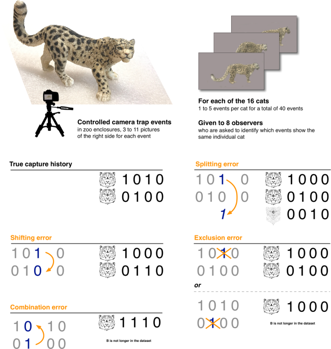
We created a photographic library containing 40 capture events, where each event contained a series of consecutive photographs from one of the 16 individual snow leopards. Each individual snow leopard was represented in one to five events (representing a range of recaptures across five sampling occasions) and the number of photographs within each event ranged from three to eleven to simulate a typical capture event (Supplementary Table S1; Fig. 1). Snow leopards have asymmetrical pelage patterns, similar to other spotted cats. This means that patterns on the animal’s left-hand side are different from those on the right-hand side. Criteria for inclusion in the library were: (i) the right-hand side of the snow leopard was displayed in at least one of the photographs, and (ii) combined with each other, the photographs showed enough of the animal’s side and were of sufficient quality to allow for individual identification. To ensure that background features could not be used to help the identification of animals, the background of all photographs was blurred using photo-editing software (Fig. 2).
Individual identification and types of error
We asked eight observers to independently identify snow leopard individuals from the 40 events by examining distinct spot and rosette patterns (Table 1; Fig. 2). Four observers were researchers with previous experience in identifying snow leopards from camera-trap photographs (‘experts’), with three of these having authored peer-reviewed papers involving abundance estimation from camera-traps. The other four observers had experience of snow leopards in captivity but not in camera-trap photographic identification (‘non-experts’). The observers performed their work independently (for the observer protocol, see Appendix S1). If an observer felt they could not reliably identify an individual from the photographs in an event, it was excluded from further classification. This reduced the number of events for some observers (<40) and in some cases the total number of individuals if all events containing a given individual were excluded (Table 1; Supplementary Table S1; Fig. 1).
To calculate the probabilities of different identification errors, we evaluated if observers correctly classified each event by scoring it as correct or incorrect (Table 1; Supplementary Table S1). Incorrectly classified events were further scored into the following categories: (1) ‘split’, meaning the event was incorrectly split from other events containing the same individual and placed by itself, thereby creating a new individual, (2) ‘combine’, where the event(s) from an individual was combined with another individual, resulting in the loss of the focal individual (with one exception, this occurred with individuals that were represented by only one event), (3) ‘shift’, meaning the event was incorrectly split from other events containing the same individual and added to another individual’s set of events but this did not result in loss of the individual (i.e. a split + combine), or (4) ‘exclude’ because the snow leopard was deemed unidentifiable. Exclusion of an event where identification is possible is a form of identification error that affects capture-recapture calculations (by placing a 0 instead of a 1 at that (re)capture event; Fig. 1); thus we included it in our analyses for assessing the total number of event errors in addition to estimating its probability. Splits are single errors that create new individuals (sometimes referred to as ‘ghosts’) from previously known individuals. Combines are single combination errors that occur when a previously-unknown individual is misidentified as a known individual (in the genetic capture-recapture literature this is also known as the ‘shadow effect’20); these reduce the number of individuals in the sample (lost). Shifts consist of two errors, a split from one individual and a combination with another. Shifts do not affect the number of individuals identified but result in erroneous identification keys that can have major implications for spatial capture-recapture methods and increase the measure of capture heterogeneity. It is important to understand what these different errors represent when estimating the probability of a splitting or combination error. Total splitting errors are thus the number of splits + shifts; while total combination errors are the number of combines + shifts (for summary see Fig. 1 and Table 1). We present separate error estimates for experts and non-experts to highlight conditions where the two groups diverge and help the interpretation of the general estimates from all observers.
Estimating observer misclassification & exclusion errors
We modelled each of the error categories (i.e. split, combine, shift, exclusion) as well as specific combinations of error categories (i.e. splitting, combination and total errors) using a logistic regression model (binomial likelihood) in a Bayesian framework run in JAGS33 within R34. This method allowed us to calculate the probability of each type of error occurring, based on the total number of events categorized by each observer (number of binomial draws, Appendix S2). Thus, for the exclusion category we consider all events as having the potential to be excluded; however for the split, shift and combine categories, we only considered the number of events that remained after the excluded capture events had been removed. We derived probability estimates not only for the general error rates, but also separate estimates for the two observer types: experts and non-experts. The advantage of using Bayesian models for these analyses was that we could directly calculate the probability that non-experts had greater exclusion, splitting or combination error rates than the experts. These resulting posterior distributions represented the difference between the two groups; thus, the proportion of the resulting posterior distribution that was above zero was the probability that non-experts were more likely to make errors than experts (the closer the proportion of the posterior distribution was to 0.5, the more likely there was no difference between the groups). We could also simulate expected values directly from the model’s likelihood function to generate the expected range of error rates from different observers in each category (see Appendix S3). For all models we used minimally-informative priors and ran a MCMC for 10 000 iterations after the chain convergence had been reached (see Appendix S3).
Estimating capture event exclusion and misclassification
We allowed the observers to exclude capture events from classification if they felt they were not confident enough to make a decision regarding the identity of an animal, as would occur in a study of images captured in the field. We allowed this option despite us creating the events with what we believed were images that could reliably classify the individual. Thus, if exclusions occurred, we hoped to gain insights into how event exclusion may be interpreted as another source of observation error. To examine whether our assumption that all 40 events were possible to identify was correct (i.e. exclusions were ‘false exclusions’), and to better understand the nature of why events might be excluded in a field study, we compared misclassification rates and exclusion rates for the eight observers for each of the 40 events. If exclusions were in fact ‘true exclusions’ because they could not be reliably matched, then we expected higher misclassifications of those events when observers did attempt to classify them.
We modelled the number of misclassification errors for individual events as a function of three factors: (1) the number of times the events were excluded by the eight observers (range 0–4; the explanatory variable we were most interested in), (2) the total number of events that belonged to that individual cat if all events were assigned correctly (range 1–5) and (3) the individual cat identity. The model had a binomial Bayesian hierarchical structure with the number of trials (max = 8) adjusted based on the number of events excluded (i.e. only events that were classified in some way could be misclassified; Appendix S3). The total number of events belonging to each individual was included to control for the possibility that correctly classifying an event may be related to the total number of events linked to each individual: for example, a cat with a single event can only be combined with another cat, whereas a cat with multiple events can be split or shifted. Also, a cat with multiple events has more reference material, so the probability of making classification mistakes may be lower than for a cat with fewer events. Individual cat ID was included as a random effect on the intercept to account for the possibility of additional variation because some cats were more difficult to classify than others (independent of the decision to exclude or not; see Appendix S3).
Impacts of splitting errors on population estimates
From each observer’s capture history we estimated the population size using a closed population capture-recapture estimation method [closedp() function from the R package ‘Rcapture’35] (Appendix S4). We used AIC to choose the highest ranking model’s population abundance estimate and compared this to the true number of animals in the population (n = 16) and also to the number of animals that were classified by each observer given that they may have excluded individuals from consideration (n ≤ 16).
To see the general effect of how misclassification of individual identities, and specifically splitting errors, within the capture history can influence population abundance estimates, we simulated snow leopard capture histories based on varying the number of capture occasions, capture probability and number of splitting errors. Because misclassification always created a net number of splitting errors (splits > combines; Table 1), this approach allowed us to investigate the general effect of how net misclassification of individual identities within the capture history influences population abundance estimates (Appendix S4 and S5). First, we simulated 1000 snow leopard capture histories based on the number of capture occasions and capture probability from our snow leopard field study in Mongolia26 and subsequently introduced splitting errors with a probability ranging from 0.5% to 25%. This was to examine how the observed rates of misidentification (between the different observers) translate into errors of population abundance estimates in our study population. Second, we simulated 1000 snow leopard capture histories for each of a variety of capture occasions and capture probabilities while introducing splitting errors (up to 5) to examine more generally how the creation of new (ghost) individual identities to the capture history influences population abundance estimates (Appendix S4 and S5).
Source: Ecology - nature.com
