Impacts of ozone and climate change on yields of perennial crops in California

County-level data in California

We use annual crop yields, harvested area, production and economic value data for 58 counties in California for the years 1980–2015 from the California County Agricultural Commissioners’ reports²¹. We analyse the 20 most valuable perennial crops in California: almonds, wine grapes, strawberries, table grapes, walnuts, hay, pistachios, navel oranges, raisin grapes, lemons, avocados, cherries, freestone peaches, nectarines, Valencia oranges, plums, dried plums, clingstone peaches, grapefruit and bushberries¹¹. These crops represent an average total production value of US$23.0 billion per year over the period of 2011–2015, accounting for more than 70% of the production value of all perennial crops in California²¹. The relationships of agricultural production, climate and ozone are analysed using historical climate and ozone data. The monthly average of the daily maximum temperature (T_MAX) and the monthly total precipitation (PRCP) at 379 stations in California are obtained from the National Weather Service Cooperative Network. Hourly ozone data at 190 sites in California from the Environmental Protection Agency’s Air Quality System³⁴ are used to calculate three widely used ozone cumulative indices designed to reflect ozone exposures on plants (that is, W126, AOT40 and SUM06)^8,24. W126 is a cumulative indicator of hourly ozone concentrations weighted by a sigmoidal scale. AOT40 and SUM06 are cumulative indicators of hourly ozone concentrations exceeding 0.04 ppm and 0.06 ppm thresholds, respectively. They are calculated as:

where O_h is the hourly ozone concentration in ppm for hour h during daylight hours (8:00–19:59), and n is the total number of hours within a period. The ozone cumulative indices are cumulated over the warm season (March to August) when ozone levels are the highest and plant growth is more likely to be affected. To adjust for missing hourly observations, similar to the correction approach suggested by the US Environmental Protection Agency³⁵, we sum the cumulative indices over the reporting hours, divide by the number of reported hours and then multiply by the total number of daylight hours within the period. To be comparable with crop data at the county level, data for sites adjacent to cropland areas within each county were averaged to produce county-wide averages. The cropland map obtained from the US Department of Agriculture National Agricultural Statistics Service³⁶ was used to limit the observations to relevant agriculture areas. Counties with less than 20 yr of data are excluded from the analysis.

Statistical yield models

On the basis of the historical data, we develop statistical yield models for each crop using the following linear regression model:

where OI is one of the three warm-season ozone cumulative indices (in units of ppm h); T_MAX,syi and PRCP_syi here are seasonal mean of daily maximum temperature (°C) and seasonal total precipitation (mm), respectively; the subscripts y, i and s are indices for year, county and season, respectively, such that T_MAX,syi is T_MAX in season s of year y in county i; β_o, β_T, β_T2, β_P, β_P2, β_CY and β_C are regression coefficients. Similar to a previous study of the temperature sensitivity of California perennials¹¹, for each harvest year we consider weather variables from the September prior to the harvest year to the August of the harvest year to account for different seasonal influences. We use seasonal average weather variables instead of monthly variables in the model to avoid too many predictor variables and thus overfitting. The four seasons are defined as autumn (September–November), winter (December–February), spring (March–May) and summer (June–August). The county-specific time trend (represented by the year term) accounts for changes in agronomic practices over time that influence yields. County fixed effects account for time-invariant factors that vary across counties, such as differences in soil quality. Similar crop models have been used in previous studies of ozone and climate^8,11.

We use the LASSO³⁷ regression method to fit the regression model, in which predictors are chosen in an automatic manner (using the ‘lars’ package in R) that is thus independent from researcher choice. The LASSO method selects a subset of predictors that explain most of the variation in outcomes by shrinking the regression coefficient towards zero, avoiding the statistical penalties of including irrelevant predictors, and is thought to improve prediction accuracy. We then perform an out-of-sample cross-validation as a robustness check, using two-thirds of the data for training (that is, model calibration), and the other one-third for testing. We compute determination coefficients (R²) between actual and predicted yields for both the training and test data. Models in which the test R² was significantly lower than the training R² indicate the risk of overfitting. CIs of R² are derived from 1,000 repeated tests with a random one-third of observations omitted.

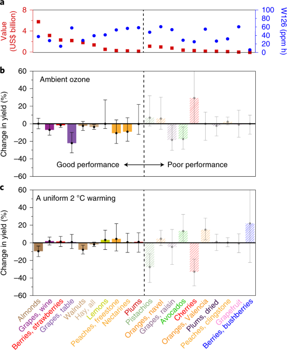
On the basis of temperature and ozone sensitivities given by the statistical yield model, we then determine the crop yield responses as percentage changes in yields. We first estimate the overall yield response to warming as the percentage difference between predictions using historical temperature and a scenario with a uniform 2 °C warming (an approximation for the magnitude of warming by 2050). Next, the impact of historical climate trends on crop yields is estimated from the difference between predictions using historical temperature and a hypothetical scenario using the 1980–2015 average temperature, to evaluate the impact of year-to-year temperature variability during 1980–2015. Similarly to Lobell and Field¹¹, we also found small sensitivities to precipitation for many crops, presumably because most crops are irrigated¹². Given the small sensitivities and large uncertainties in precipitation projections^9,12, we focus our analysis of climate change on the temperature effects. The yield effect of ambient ozone is estimated from the percentage differences between predictions using historical ozone levels and a hypothetical scenario with zero ozone (which has been used in other studies)^3,6,8. To get state-wide average yields, yields are weighted by the harvested area of each crop in each county. To analyse regional differences, we also gathered counties into eight agricultural districts. The definition of agricultural districts is consistent with the California County Agricultural Commissioners’ reports (Supplementary Fig. 2).

Finally, to determine the CIs related to these estimates, we use the bootstrapping method³⁸ to produce distributions by using a set of crop models generated from resampling (with replacement) the observations 1,000 times, and the 2.5th and 97.5th percentiles from the 1,000 bootstrap replicates are selected as 95% CIs. By selecting new predictors for each replicate, the bootstrapping method accounts for uncertainties in model formulation.

Future projections

On the basis of the crop models we developed, we combine historical sensitivities with future projections of ozone and climate to assess their potential impacts on yields to 2050. The future projections assume no new adaptation between now and then, or holding technology equivalent to current levels (2001–2010), so that the effects of changes in ozone levels and climate on future yields can be isolated. Two RCP scenarios (RCP4.5 and RCP8.5) are used to represent a range of policy options regarding ozone regulation and climate adaptation. RCP8.5 represents a business-as-usual scenario in which mean global temperatures increase by >4 °C (ref. ²⁶), while RCP4.5 represents a mitigation scenario with moderate ozone regulation that is likely to limit the increase of mean global temperature to ~3 °C (ref. ²⁷).

We use decadal projections of regional air quality and climate over the US for current (2001–2010) and future (2046–2055) decades at a 36-km resolution simulated by the Weather Research and Forecasting Model with Chemistry (WRF/Chem)^30,39, downscaled from the North Carolina State University’s version of the Community Earth System Model (CESM_NCSU)^40,41,42. Future predicted air quality takes changes in both emissions and climate into account. The gridded data are aggregated to the county level by calculating the average of all the grids classified as cropland areas within each county. Climate and air quality data are bias-corrected to ensure that they are consistent with the observations used in model calibration. For the climate data, following Bruyère et al.⁴³, seasonal mean biases between simulations and observations by county are calculated and then subtracted from the original simulations for both current and future years to generate the bias-corrected data. We corrected the simulated ozone exposures in each county by multiplying the ratio of observed/simulated ozone levels in current years as has been done in previous similar studies⁴. The simulated data at county level are combined with statistical yield models to predict yields of each county, assuming the current technology. State-average yields are calculated by assuming the current crop area distribution. To obtain CIs related to crop model uncertainty, the yield projections are repeated 1,000 times by using a set of crop models generated from bootstrap samples of historical observation data.

Reporting Summary

Further information on research design is available in the Nature Research Reporting Summary linked to this article.

Source: Ecology - nature.com