Integrating multiple sources of ecological data to unveil macroscale species abundance

A framework to estimate macroscale species abundance

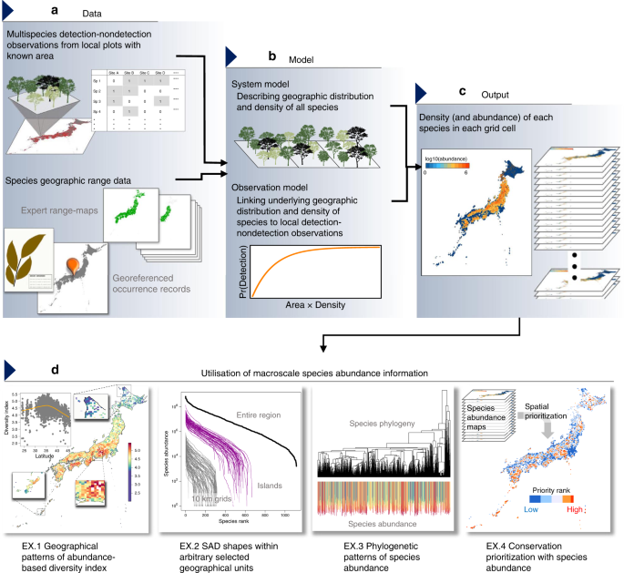
In the following sections, we describe a hierarchical modelling approach that estimates species abundance in discrete geographical units (e.g. grid cells) from spatially replicated multispecies detection–nondetection observations, in combination with various data sources indicating the geographic distribution of species (Fig. 1). A hierarchical model is composed of a series of submodels, including an observation model describing the distribution of data conditional on some latent state variables and a system model describing the variation in the state variables^14,15,16. In the following, we first describe a generalised linear mixed model (GLMM), which explains the multispecies detection–nondetection observations in terms of individual density of each species, and therefore explicitly links binary observations to underlying species abundance. Then, we extend this model to incorporate other sources of information about species occurrence that facilitate the inference of abundance for a number of species over a large geographical extent. To describe the basic modelling idea, we here illustrate the models in their simplest form, which includes only intercept and independent random effect terms. The specific, more complex model that we used in our application is described in the later section.

A model for spatially replicated detection–nondetection data

We assume that there is a set of geographic areas of interest that contain I species of interest and are divided into J geographical grid cells. Suppose that grid cell j(j = 1, …, J) contains K_j > 0 replicated sampling plots in which occurrence was assessed for each species. We denote detection (1) or nondetection (0) of species i in plot k in grid cell j as y_ijk (i = 1, …, I; j = 1, …, J; k = 1, …, K_j). We also assume that the area of each sampling plot was recorded, and denote the area of sampling plot k in grid cell j as a_jk.

The goal of the inference is to estimate the abundance of each species within each grid cell from these locally replicated detection–nondetection observations. To achieve this, we explicitly make several key assumptions in the data generating process. First, we assume that individuals are distributed within some suitable habitats (e.g. forests) in which sampling plots are placed so that they never overlap. The area of suitable habitat is supposed to be known for each grid cell j, which we denote as A_j. Second, we assume that for each grid cell the spatial point pattern of individuals within the habitats can be regarded as an independent superposition of homogeneous Poisson point processes, each of which represents the spatial alignment of individuals of a species. In the ecological context, this assumption implies that the centres of individuals are regarded as points, and individuals are distributed independently of one another with species-specific individual densities that are constant within a grid cell⁴⁸.

These assumptions give us a probability function that explicitly links the probability of species detection within a plot to the density of that species in the grid cell. Let us denote the individual density of species i in grid cell j by d_ij. Then, the number of individuals occurring in a plot of area a_jk independently follows a Poisson distribution with a mean of d_ija_jk⁴⁸. Therefore, the probability for detecting at least one individual of species i in plot k in grid cell j, p_ijk, can be written as

where (exp (-{d}_{ij}{a}_{jk})) corresponds to the probability mass of a Poisson distribution with a mean d_ija_jk at zero (i.e. a probability that the plot captures no individuals).

On the basis of these settings and assumptions, we provide a state space formulation of the first hierarchical model we consider, in which the model is described in terms of a series of submodels that are conditional on latent state variables and parameters^14,15,16. The latent variable of the model was the cell-level individual density of species, which we have already defined as d_ij.

The observation model describes the occurrence of species within a sampling plot. We can regard the detection–nondetection observation of species, y_ijk, as a random variable that independently follows a Bernoulli distribution with a detection probability p_ijk:

where p_ijk is determined by Eq. (1) under the assumption of the superposed homogeneous Poisson point process.

The system model describes variation in the individual density d_ij. We decompose the logarithm of d_ij into an intercept term μ and three normally distributed random effects, species ({e}_{i}^{(1)}), grid cell ({e}_{j}^{(2)}), and the combination of species and grid cell ({e}_{ij}^{(3)}):

These submodels jointly construct a Bernoulli GLMM with complementary log–log link, in which a_jk is treated as an offset term. The model can therefore be fitted to data with standard GLMM packages that implement multiple random effects, such as lme4 in R⁴⁹.

We note that, in practice, the size of the geographical units must be determined arbitrarily. Because the model assumes a constant individual density within each unit and the density is determined via replicated detection–nondetection observations, there is a trade-off along the size of the units. Thus, establishing smaller geographical units is likely to increase the likelihood of an inference conforming to the modelling assumption by reducing environmental heterogeneity and hence variation in individual density within the units. However, this comes at the expense of an increased computational burden and a less accurate estimation of individual density. This is because the number of geographical units will be increased for a given spatial extent, and thus the number of random-effect terms will also increase while decreasing the number of replicated plots within the units. Conversely, establishing larger geographical units will ensure a larger number of replications and fewer random effects but will also increase the likelihood of violating the modelling assumptions. Therefore, the size of geographical units should be carefully determined depending on the details of each application.

In addition, it should be remembered that the estimation of individual density relies on the assumption of the superposed homogeneous Poisson point process that was made for modelling convenience rather than for ecological plausibility, and that its violation can result in a biased inference. Specifically, spatial clustering of individuals (i.e. aggregated distribution) may lead to an underestimation of individual density because it inflates the probability of nondetection of species within a sampling plot^46,47. Even when the assumption of the superposed homogeneous Poisson point process holds, the individual density of species can be underestimated or overestimated when the plots were selectively placed to sample or avoid specific species. Furthermore, the Poisson point process assumption implies that individual density may not be adequately identified when the individual density or the area of sampling plot, or both, is significantly high because the derived detection probability (Eq. (1)) approaches 1 as d_ija_jk increases. This suggests a possibility that, under the random effect formulation where the estimates are shrunk towards the average¹⁵, the underlying individual density and sampling design (i.e. specification of the area of plots) can interact to cause underestimation of abundance, especially for dominant species.

Integrating cell-level occurrence information

Because information is shared over species and grid cell by random effects, the model described above can provide estimates of individual density that are specific to each species and cell. However, the estimates may be inaccurate, especially in grid cells where the number of plots is limited and species density is low. Moreover, the model does not explicitly account for the “zero-inflated” nature of species abundance, which assumes that individual density of species is structurally zero in the region outside the species range. To overcome these issues, we extend the model to integrate replicated detection–nondetection observations with data that may directly inform about the cell-level presence–absence of species, such as species occurrence records and expert range maps.

We introduce a latent indicator state variable that represents the cell-level presence–absence of species and is denoted as z_ij. The detection probability p_ijk is then expressed as follows:

which indicates that the detection probability is 0 when the species is absent in the cell (z_ij = 0), but it takes (1-exp (-{d}_{ij}{a}_{jk})) when the species is present in the cell (z_ij = 1). Hence, d_ij now represents the individual density that is conditional on the presence of that species.

We regard z_ij as a random variable following a Bernoulli distribution and add an additional system model component to describe it. By adopting a similar modelling approach applied for the conditional individual density (Eqs. (3)–(6)), the additional components can be constructed as follows:

where ψ_ij is the occurrence probability of species i in cell j, which was decomposed into an intercept term η and two normally distributed random effects that vary over species ({u}_{i}^{(1)}) and cells ({u}_{j}^{(2)}) on a logit scale.

We assume that the cell-level species occurrence z_ij is partially observed via the plot-level detection–nondetection observations and/or the auxiliary cell-level presence–absence information that is independent of the detection–nondetection observations. A cell-level presence of species may be registered, for example, by museum-based or herbarium-based specimens and/or occurrence records, while absence of species may be deduced by exploiting, for example, expert range maps⁵⁰ and/or regional species checklists. In general, the information about the species absence should be treated conservatively because it is difficult to verify⁵⁰; therefore, the evidence of species presence should be prioritised when different sources of data are in conflict.

Technical details of the inference of this integrated model are described in Supplementary Note 1. We note that this model even enables us to utilize geographical grid cells that contain no detection–nondetection observations but have cell-level presence–absence information for some species (see Supplementary Note 1).

Ecological variables obtained as derived quantities

Once estimates (or posterior samples, in case of fully Bayesian approach) of random effects are obtained, we can derive the estimates of ψ_ij and d_ij, denoted by ({hat{psi }}_{ij}) and ({hat{d}}_{ij}), respectively, by substituting the estimates of random effects into Eqs. (9) and (3), respectively. Based on these estimates, we can further derive estimates for a wide array of variables that are of ecological interest. For example, let us use m_ij = 1 to denote that the value of z_ij is known (through either the detection–nondetection observations or the cell-level occurrence information) for species i in cell j and m_ij = 0 denotes otherwise. Then, the number of modelled species that are actually present in cell j, denoted by S_j, can be estimated as

Note that the use of the estimated occurrence probabilities (hat{psi }) enables this estimator to account for the possibility of the presence of species even when they are not detected in the replicated plots (cf. ref. ⁵¹) or no detection–nondetection observation is available in the grid cell. Let N_j denotes the vector of abundance of all species in cell j, the property of an ecological community that we aimed to infer, and can be estimated for each grid cell as

where as defined above, A_j denotes the area of habitats in cell j. We can also estimate the species abundance for a subset of the area of interest ({mathcal{J}}), denoted by ({{bf{N}}}_{{mathcal{J}}}^{* }), as follows:

Note that the estimates of abundance of each species further permit to obtain various diversity indices that are a function of a vector of (relative) abundance, such as Shannon entropy and Gini–Simpson index, as well as other generalised metrics including phylogenetic/functional diversity indices and the Hill numbers⁵². In addition, the total area of occupancy within the modelled geographic areas, denoted by R, can be estimated for each species as follows:

Model variants

The above model has the most trivial form in the sense that the variation in individual density was explained only by several unstructured random-effect components that share information across all grid cells and species^53,54,55. It can be extended, however, in various ways to accommodate additional complexities. For example, in an analogous fashion to many other classes of hierarchical models and species distribution models (SDMs), environmental covariates could be introduced in the system model to explicitly describe the association between environmental factors and individual density. The model could also explain the correlation structure of random effects on the geographic and/or phylogenetic space in an explicit manner^56,57. Additionally, the correlation between random effects for conditional density (e) and that for occurrence probability (u) could be accounted for, as shown in the following application. Such generalisations will potentially enhance the model prediction and provide further ecological insights. Nevertheless, some of these extensions may be difficult to adopt in practice, especially in studies that examine a very large number of species and grid cells, as is the case with our application described below, because the model may involve an excessive number of parameters and/or a huge covariance matrix, rendering the inference computationally challenging⁵⁴.

Woody plant communities in East Asian islands

We applied the proposed framework to a dataset of woody plant communities in mid-latitude forests in Japan. For the replicated detection–nondetection observations, we compiled a large dataset from vegetation surveys that consists of 40,516 georeferenced plots which comprises the dataset of Kusumoto et al.⁵⁸ and the national vegetation survey of Japan (http://www.biodic.go.jp/english/kiso/vg/vg_kiso_e.html). These plots were placed in natural forests in various successional stages between 24°02′–45°30′N and 122°56′–153°59′E (Supplementary Fig. 1a). The plot area ranged from 0.01 to 18,000 m² where the typical size was about 100 m² (Supplementary Fig. 1b). The time period of the surveys spans from 1954 to 2013, in which a substantial proportion of data have been collected between the 1970s–1980s and 2000s–2010s (Supplementary Fig. 1c).

In the vegetation survey, species occurrence in the sampling plots (called “relevés”) is traditionally recorded according to cover classes for individual species at every different layer. We converted these vegetation observations into detection–nondetection records by assigning 1 if the species appeared in the plot and 0 otherwise. In this analysis, we standardised the names of woody plant species and pooled the data for varieties and subspecies with those of their parent species following a list of Japanese plant names⁵⁹. As a result, we obtained detection–nondetection observations for 1248 species, which includes introduced species and covers almost every woody plant species found in Japan.

It should be noted that as the survey is based on the measurement of plant cover, species occurrence can be recorded regardless of the size of individuals within a plot. This implies that in the following analyses, estimates of species abundance nominally encompass individuals of any size, including seedlings (but not seeds), that are observable and identifiable during the survey. In addition, in the vegetation survey, species can be recorded even when their stems are absent from the plot, and some branches are hanging over the plot. In terms of the Poisson point process assumption of the model, this implies that the area of the plot is effectively enlarged, so that some individuals located outside the plot can be detected. Therefore, the use of the cover data can lead to a positive bias in the inference of species abundance, especially for large tree species. Such a bias may become less relevant, however, in plots with a larger area, which have smaller margins relative to their area.

We divided the entire study area into 10 × 10 km grid cells^37,60. We analysed in total 4619 cells, which covered ca. 99.2% of the total land area of Japan. In total 3683 cells contained at least one vegetation plot.

We also compiled the species occurrence information at a cell level based on multiple data sources that were independent of the vegetation survey dataset. Species presence was registered from museum and herbarium specimens, species occurrence records, and distribution maps of plant species compiled by Horikawa⁶¹. Species absence was recorded from the distribution maps⁶¹ and regional species checklists compiled by prefectures of Japan³⁶.

Model fitting and inference

As a preliminary analysis, several model variants were fitted to these data using the maximum marginal likelihood procedure and then compared based on AIC and three other benchmarks of predictive performance that we described below. The preliminary models included a model without data integration, a model with data integration, a model with correlated random effects, and several models with covariate effects. Details of this preliminary analysis are described in Supplementary Note 2. As a result, an integrated model with two cell-specific covariates, AET, and the HII⁶², along with their interaction effect and correlated random cell effects, was selected as the best model and used in the following analyses. Specifically, the model is specified by a series of equations as follows:

where x_1j and x_2j, respectively, represent the values of AET and HII in cell j, scaled to have mean 0 and variance 1. Note that the correlation between the two cell random effects, ({e}_{j}^{(2)}) and ({u}_{j}^{(2)}), is accounted for by specifying a bivariate normal distribution with an additional correlation parameter ρ. A 10-fold cross-validation was conducted to asses the goodness of fit of the model to replicated detection–nondetection observations in which the mean area under the curve (AUC) for validation datasets was estimated as 0.894 (standard deviation: 0.001). To calculate the AUC, we omitted data where the absence of species was indicated by the auxiliary species occurrence information to exclude trivial predictions for structural zeros.

Based on the estimates of the selected model, the abundance and area of occupancy of 1248 woody plant species within natural forests was estimated for 4619 grid cells by using Eqs. (13) and (15), respectively. The area of natural forest in each cell was obtained based on the national survey of the natural environment (http://www.biodic.go.jp/trialSystem/EN/info/vg.html).

The uncertainty associated with the estimates of species abundance, area of occupancy, and quantities obtained as a function of these were evaluated by using the parametric bootstrap procedure for hierarchical models⁶³ in which 100 bootstrap samples were obtained to measure the standard error of each estimate. To accommodate reduced uncertainty in the geographic distribution of each species (i.e. z_ij) due to the availability of the auxiliary cell-level presence–absence information, the bootstrap procedure was conducted with the auxiliary dataset being fixed.

Validation

The estimates of species-specific individual density were validated based on data from geographically replicated forest inventory plots that were independent of the fitted data. We used three sources of forest inventory data that were collected in natural forests in Japan. They include the forest dynamics plots (FDP), the national forest inventory plots (NFI), and forest sampling plots along latitudinal and elevational gradients (FSLE). Sampling procedures and spatial coverage differed between the inventory data as we explain below.

The FDP dataset consists of species abundance data collected from 40 quadrats. In each quadrat, which was usually 1 ha in size, individuals with a diameter of approximately  >5 cm at breast height (DBH) were monitored⁶⁴. This dataset fairly represents the mosaic structure of forests with different developmental stages and thus is expected to precisely capture local population size for common climax species in old growth mountain forests, while it may poorly represent the population of pioneer or fugitive species, especially in lowland forests. The FDP dataset is publicly available from the Biodiversity Center of Japan (http://www.biodic.go.jp/moni1000/findings/data/index_file.html).

The NFI dataset included 7672 plots in which woody plant individuals were assessed in nested concentric circular plots. Individuals with DBH  >1 cm were measured in a 0.01 ha circular area, while those with DBH  >5 and  >18 cm were surveyed in a 0.04 and 0.1 ha circle, respectively (http://www.rinya.maff.go.jp/j/keikaku/tayouseichousa/). The NFI plots were systematically placed in a 4 km × 4 km grid laid over entire Japan and thus were expected to provide less-biased samples of density of woody plants. The NFI dataset is publicly available from the Forestry Agency of Japan (http://www.rinya.maff.go.jp/j/keikaku/tayouseichousa/chousadeta.html).

The FSLE dataset included 460 plots placed within climax forests in five regions (central and western Hokkaido, Shizuoka, Miyazaki, and Kagoshima prefectures) in Japan (unpublished data by Y. Kubota). For each region, abundances of woody plants were surveyed along an elevational gradient in which 10 replicated plots were located for each 100–200 m elevation interval. For each plot, woody plant individuals larger than 2 m in height were counted over a 0.01 ha area. The sampling design along both the elevational and latitudinal gradients was expected to well reflect the environmental heterogeneity in the mid-latitude forests.

For each dataset, the species abundance data were pooled within each grid cell and compared to the model prediction to estimate root mean square error and bias in the prediction of individual density, in addition to the correlation between observation and prediction on a log–log scale. For each grid cell, observed and predicted individual density were compared for all species, except for the species whose absence in the cell is indicated by the cell-level occurrence information. In order to predict the abundance in NFI plots, we set the area of each plot to 0.1 ha.

Additionally, prediction of the total individual density was validated with a global estimate of tree density¹⁷, which here we call the global map of forest trees (GMFT). The GMFT provides the density of trees with DBH  >10 cm at 1-km² resolution that was predicted based on regression models for forested areas in 14 biomes¹⁷. The GMFT estimates are provided in the raster format and are publicly available (https://elischolar.library.yale.edu/yale_fes_data/1/). The GMFT estimates were matched to the grid specification adopted in this study to obtain the individual density per grid cell, which was then converted to the individual density per 1 km² natural forest by dividing with the area of natural forest for each cell. Because GMFT does not distinguish natural and planted forests, the GMFT estimates were scaled for each cell by the proportion of the area of natural forest to that of the entire forest (i.e. both natural and planted forests) within the cell to correct GMFT estimates for natural forests. The area of planted forest in each cell was obtained based on the national survey of the natural environment (http://www.biodic.go.jp/trialSystem/EN/info/vg.html). The corrected GMFT estimates were used to validate the prediction of individual density in each cell, in the same manner as the validation with forest inventory data; they were also used to obtain the total woody plant abundance within the natural forests in the entire region. We note that although there was an alternative GMFT that was based on regression models in 813 ecoregions, the results of validation were quantitatively similar to that with the biome models.

Additional details of the validation can be found in Supplementary Note 2.

Inference of macroevolutionary processes in metacommunities

The UNTB⁵ provides a mechanistic explanation of the origin and maintenance of biodiversity; based on the premise that all individuals in a system are functionally equivalent and thus follow neutral processes of demography, dispersal, and speciation, the UNTB derives SADs, at both local-community and meta-community (i.e. species pool) scales, in addition to a range of other macroecological and macroevolutionary patterns such as the species–area relationship⁴⁰, β diversity⁶⁵, and various phylogeny characteristics⁶⁶.

The UNTB bridges evolutionary biology and community ecology by linking, theoretically, macroevolutionary processes to biodiversity patterns. In particular, it predicts that the statistical form of the SAD in the metacommunity is dependent on the mode of speciation^{5,11,12,18,19,20}. The point mutation speciation model, which formed the basis of the first UNTB proposed by Hubbell⁵, models speciation as a process in which each new species is represented initially by a single individual. The point mutation speciation model predicts a metacommunity SAD that follows the logseries distribution, a distribution that is characterised by a relatively high proportion of rare species^5,21. In contrast, the random fission speciation model assumes that speciation occurs in the metacommunity owing to the random division of a population of an existing species^12,19. The random fission speciation model predicts a fairly even metacommunity structure, which is related to the MacArthur’s⁶⁷ broken-stick model^12,19. The point mutation speciation and random fission speciation models represent the two extremes of a spectrum of speciation modes in UNTB. This spectrum of speciation modes has been argued to be unified with the concept of protracted speciation, which characterises speciation as a gradual, drawn-out process^11,20. The UNTB with protracted speciation predicts a metacommunity SAD that follows a difference-logseries distribution. The difference-logseries distribution follows a logseries distribution at large abundances, while behaving differently at small abundances; namely, it predicts fewer rare species than the logseries distribution^11,20.

Our ability to infer evolutionary processes that underpin observed biodiversity patterns is, however, fundamentally limited because species abundance data can be obtained only from local communities. Indeed, earlier studies have shown that differences in the mode of speciation are hardly discerned based on samples from local communities as they may not leave a signature on SADs realised in dispersal-limited localities^5,11,12,18. The limitation in data acquisition also prohibits us from identifying the rate of speciation (ν) from SADs because local community SADs are determined by the fundamental biodiversity number (θ), which is a compound parameter depending both on ν and the metacommunity size (J_M)^12,21; but see ref. ¹⁸. Consequently, fundamental macroevolutionary properties of a metacommunity, such as ν and the average lifespan of the species (L²⁹), have remained largely unknown.

Although defining a metacommunity is difficult in practice, discerned biogeographic divisions will approximate its theoretical definition, as they can be regarded an evolutionary unit within which most member species spend their entire evolutionary lifetimes⁶⁸. Based on a previous biogeographic assessment of woody plants in the Japanese archipelago³⁶ and Takhtajan’s floristic provinces⁶⁹, we thus divided the archipelago into four ecoregions that belong to different biogeographic divisions (Fig. 4) and obtained metacommunity SADs by aggregating abundance estimates over grid cells within each ecoregion (Eq. (14)). The four ecoregions are defined as follows: (1) The central continental arc region is the largest ecoregion, which includes the three largest islands in Japan (Honshu, Shikoku, and Kyusyu). It encompasses deciduous and evergreen broad-leaved forests and belongs to the Takhtajan’s Japan–Korea province; 3478 geographical grid cells belong to this ecoregion. (2) The northern continental arc region is the second largest ecoregion, and it includes Hokkaido, the second largest island of Japan. It encompasses coniferous and deciduous broad-leaved forests and belongs to the Takhtajan’s Sakhalin–Hokkaido province. The Tsugaru Strait separates the central continental arc region and northern continental arc region; 986 geographical grid cells belong to this ecoregion. (3) The southern continental arc region is composed of the Nansei Islands and separated from the central region by the Tokara Strait. It encompasses evergreen broad-leaved forests and belongs to the Takhtajan’s Tokara–Okinawa province. This ecoregion comprises 138 geographical grid cells. (4) The oceanic islands region is composed of the Bonin (Ogasawara) Islands. It encompasses evergreen broad-leaved forests and belongs to the Takhtajan’s Volcano-Bonin province. Differing from other ecoregions, in which almost all the lands are continental islands, the oceanic region is composed of oceanic islands only. It includes 17 geographical grid cells.

For each ecoregion, we fitted and compared three variants of the UNTB to the estimate of the metacommunity SAD. The fitted model includes the point mutation speciation model^5,21, the random fission speciation model¹², and the protracted speciation model¹¹; for each of these models, a probability function of the metacommunity species abundance vector (i.e. likelihood function for metacommunity SAD) and/or an analytical solution of the SAD in the stationary metacommunity has been obtained and can be used for model fitting.

The point mutation speciation model was fitted to the metacommunity SADs by using maximum-likelihood method. The likelihood function for metacommunity SAD (i.e. assuming no dispersal limitation) under point mutation speciation model is known as the Ewens sampling formula (e.g. Eq. (2) in ref. ²¹). Formal likelihood-based inferences were, however, difficult to obtain for the other two models. Although a sampling formula has been acquired for a metacommunity under random fission models (Eq. (38) in ref. ¹²), we were not able to apply this formula to our specific data as it underflows when the size of metacommunity is large, even when high precision arithmetic is used. We thus reached a compromise to use Eq. (21) in ref. ¹², which was derived without considering the sampling process, but provides the equilibrium probability function of the species abundance vector in a metacommunity with a fixed size J_M. For protracted speciation model, no likelihood function was available. To fit this model, Rosindell et al.¹¹ used “composite likelihood” that was suggested by Alonso and McKane⁷⁰. This approach was however not practical in our case because of the large metacommunity size, thereby requiring an excess number of evaluations of the expected number of species with specific abundance. This prohibited its adoption in the numerical optimisation procedure. We therefore applied a least-square method to the Preston’s abundance octaves of metacommunities. We note that in addition to these three models, we also fitted the per-species speciation model of Etienne et al.¹⁸. However, this model consistently yielded boundary estimates that made the model identical to the point mutation speciation model. We thus omitted it from the comparison.

These differences in the fitting procedure render the model comparison complicated. To compare fitting of the models, while accounting for differences in the number of parameters (we note that point mutation model and random fission model have one free parameter (θ) but protracted speciation model has two (θ and β)), we prefer to use information criteria^9,71 which relies on the formal maximum-likelihood inference⁷². However, to fully utilise this approach was impossible in our application because the likelihood function was available only in the point mutation model. Thus, we compared the models based on the Akaike information criterion (AIC) and the Akaike weights⁷³ calculated with “composite likelihood”⁷⁰, assuming that the parameter estimates of the random fission speciation model and protracted speciation model attain the maximum likelihood. In the model comparison, we also included a Poisson-lognormal mixture model⁷⁴ as a flexible, simple baseline statistical model⁹.

The objective function (i.e. negative log-likelihood or sum of squared error) of the variants of UNTB was minimised in terms of fundamental biodiversity number θ (in addition to β, in the case of protracted speciation model). Estimates of the speciation rate ν (per individual per generation) and mean species lifetime L (generations) were then derived as a function of these estimated parameters and metacommunity size J_M (individuals). In point mutation model, ν relates to other quantities as (theta =frac{nu }{1{,}-{,}nu }({J}_{{rm{M}}}-1))²¹, whereas in random fission model, the relationship is given as (theta =sqrt{nu }{J}_{{rm{M}}})¹². In the protracted speciation model, the corresponding equation is given as (theta =frac{mu }{1{,}-{,}mu }({J}_{{rm{M}}}-1)), where μ = (1 + τ)ν and (tau =frac{{J}_{{rm{M}}}-1}{beta }-1)¹¹. The average species lifetime is obtained from the general equation of Ricklefs²⁹: (L=frac{{rm{equilibrium}} {rm{number}} {rm{of}} {rm{species}} {rm{in}} {rm{metacommunity}}}{{rm{rate}} {rm{of}} {rm{production}} {rm{of}} {rm{new}} {rm{species}}}). The corresponding formula is as follows: for point mutation speciation model, (Lapprox -mathrm{log},nu); for random fission speciation model, (Lapprox {nu }^{-frac{1}{2}})¹²; for protracted speciation model, (Lapprox -tau mathrm{log},tau mu)¹¹.

National red list categories of species in Japan

We categorised each woody plant species based on the 2019 version of the national red list of Japan. The national red list of Japan adopts categories of threatened species modified from the IUCN Red List (http://www.biodic.go.jp/english/rdb/rdb_f.html). Specifically, the current national red list classifies species into categories compatible with the IUCN Red List (CR, EN, VU, NT, and DD) when they are judged to be at risk of extinction, although it does not have specific categories that correspond to Least Concern (LC) and Not Evaluated (NE) in the IUCN Red List. These two statuses are therefore not distinguishable in the national red list. For this reason, we pooled all species with such status (i.e. species that could not be classified to the at-risk categories), which were collectively labelled as “not classified (NC)”.

In the analysis described in Implications for biodiversity conservation, we omitted 130 introduced species that are outside the scope of the national red list. In addition, we ignored red list categories of subspecies or variant species because we have aggregated these taxa to their parent species in the preceding model fitting procedure (see Woody plant communities in East Asian islands).

Reporting summary

Further information on research design is available in the Nature Research Reporting Summary linked to this article.

Source: Ecology - nature.com