Mutualism increases diversity, stability, and function of multiplex networks that integrate pollinators into food webs

Network architecture

We created multiplex networks (Fig. 2) by generating food webs using the “niche model” (Fig. 2a) parameterized with 50 species (S_f = 50) and 10% directed connectance (C_f = L_f/S_f² = 0.1, where L_f is the number of feeding links)⁴⁸. The niche model stochastically assigns each species i three traits: (1) a niche value (n_i) drawn randomly from a uniform distribution between 0 and 1, (2) a feeding range (r_i) where r_i = xn_i and x is drawn from randomly from a beta distribution with expected value 2C_f, and (3) a feeding center (c_i) drawn randomly from a uniform distribution between r_i/2 and min(n_i, 1 – r_i/2). Species i feeds on j if n_j falls within i’s feeding interval [c_i – r_i, c_i + r_i]. We selected niche-model food webs with 0.0976 < C_f < 0.1024 that were comprised of 50 species (S_f = 50), of which exactly 20 were plants and five were herbivores that only feed on plants (i.e. have trophic level [TL] = 2), yielding 102 food webs. We also generated plant−pollinator networks using a stochastic model⁴⁹ with 3−19 plant-with-pollinator species (P) and exactly twice as many animal−pollinator species (A = 2 × P) to maintain pollinators’ average resource availability in networks of increasing diversity. This yielded approximately 14 networks within each of 17 diversity classes ranging from 9 to 57 species (S_p = P + A = 9, 12, …, 57) for a total of 14 × 17 = 238 plant−pollinator networks that covered the empirically observed range of nestedness (Fig. 2b, see Supplementary Methods for more details). We constrained the number of pollination links (L_p) to ensure that pollination connectance (C_p = L_p/PA) broadly decreased as S_p increased in an empirically realistic manner (Supplementary Fig. 1a). We integrated each of the 238 plant−pollinator networks with one of the 102 food webs yielding N = 238 × 102 = 24,276 networks of increasing species diversity (S = S_f + A = 56, 58, …, 88). We did this by randomly choosing P of the 20 plant species already in the food web and assigning the A pollinators to those P plant species as determined by the plant−pollinator network (Fig. 2c). This left 20 – P plant species without pollinators.

We linked pollinators to consumers in the food web in Rewards Only (RO) treatments by setting each pollinator’s n_i to ±5% of the n_i of a randomly selected strict herbivore (TL = 2) from the food web (Fig. 2d). Pollinators’ r_i and c_i were set to zero. This causes pollinators to be preyed upon by predators similar to predators of herbivores and to consume only floral rewards as determined by the plant−pollinator network. Because the connectance (C_p) of our simulated plant−pollinator networks decreases with increasing diversity (S_p) and pollinators have no other resources, connectance (C = L/S², where L is the total number of links) decreases on average from 0.091 to 0.06 as initial species diversity (S) increases from 56 to 88 in the RO multiplex and corresponding Food Web (FW) treatments (Supplementary Fig. 10). In the Rewards Plus (RP) treatments (Fig. 2e), we set each pollinator’s n_i, r_i and c_i to ±5% of the corresponding n_i, r_i and c_i of a randomly selected herbivore or omnivore that eats plants (2 ≤ TL ≤ 2.3). The RP treatment links herbivorous and omnivorous pollinators to food webs (Fig. 2c), which maintains a constant average connectance (C = 0.102) with increasing S (Supplementary Fig. 10). Feeding on both vegetation and floral rewards of the same plant species allows two links between plants and pollinators in RP networks. The corresponding FW treatment has slightly less C than the RP multiplex network because the FW eliminates the link to rewards and maintains only the herbivory link (Fig. 2d, Supplementary Fig. 10). We ignore this issue to simplify comparisons between all treatments.

Overall, as initial species diversity (S) increases (Fig. 4a), plants with pollinators in the multiplex networks increase from 3 to 19 of the 20 total plant species and mutualistic interactions increase from directly involving 16−65% of species in the networks. Correspondingly, initial herbivory in Food Web (FW) treatments increases from directly involving approximately half to three quarters of the species in the networks. We thus analyze how outputs vary with increasing initial diversity, which corresponds to increasing prevalence of mutualism in multiplex treatments or increasing herbivory in FW treatments.

Network dynamics

To model multiplex dynamics, we extended ATN theory^16,18,20,51 by integrating a consumer-resource approach to pollination mutualisms in which pollinators feed on floral rewards (R) and plants consume reproductive services produced by plants^30,31. Plants benefit from pollinators depending upon on the quantity and quality of pollinators’ visits in terms of the rate at which pollinators consume plants’ rewards and the fidelity of pollinators’ visits to conspecific plants^30,31. Pollinators in RP treatments also feed on species’ biomass according to ATN theory.

More specifically, ATN theory models the change in biomass B_i over time t for consumer i as

where x_i is the allometrically scaled mass-specific metabolic rate of species i and e_ji is the assimilation efficiency of species j eating i. C_ij is the rate of species i assimilating B_j, the biomass of species j:

where y_ij is the allometrically scaled maximum metabolic-specific consumption rate. F_ij(B_j) is the functional response for i eating j:

where ω_ij is i’s relative preference for j, h is the Hill coefficient⁷¹, and B_0ij is the “half-saturation” density of resource j at which i’s consumption rate is half y_ij¹⁸. The form of the preference term, ω_ij, determines if a trophic generalist (i) is treated either as a “strong generalist” (ω_ij = 1) or “weak generalist” (ω_ij = 1/(num. species in i’s diet)⁷². Here, we present results only for weak generalists that search for each of their resources equally even if one or more of their resources are extinct. Equation 3 is a Type II functional response when h = 1 and a Type III response when h = 2. We use h = 1.5 for a weak Type III response⁷¹.

We use ATN theory’s logistic growth model¹⁸ to simulate biomass dynamics of plants without pollinators as:

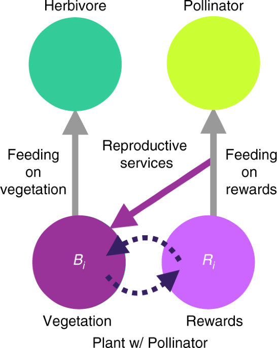
where r_i is the maximum mass-specific growth rate of plant i, and K is the carrying capacity of the plant community. For plant with pollinators i (Fig. 1), we model its vegetative biomass dynamics as:

and the dynamics of its floral rewards biomass as:

where β_i is the production rate of floral rewards, s_i is the self-limitation rate of floral reward production, and κ_i is the cost of producing rewards in terms of total vegetative growth. P(R_i) is the functional response describing how benefit to i accrues due to reproductive services provided by i’s pollinators:

which is a function of the quantity and quality of pollination provided by pollinator j. Quantity is j’s consumption rate on i’s floral rewards. Quality is j’s consumption of i’s rewards as compared to j’s consumption of all the resources it consumes. Quality is therefore j’s relative consumption rate of i’s floral rewards, a measure of j’s fidelity that ensures more specialist pollinators typically provide higher quality services than generalist pollinators by, for example, depositing higher concentrations of conspecific pollen³⁰. The form of the functional response describing benefit accrual due to animal-pollination (f) reflects the assertion that reproductive services saturate⁵³ at 1 according to: reproductive services/(0.05 + reproductive services). As P(R_i) approaches 1, the realized growth rate of plant with pollinators i’s vegetative component approaches r_i, its maximum growth rate.

Pollinators follow the dynamics typical of ATN consumers (Eq. 1) with the exception that they access rewards biomass R_i instead of B_i in RO treatments (Eq. 8) or in addition to the biomass of other resource species (Eq. 9) in RP treatments:

Parameterization

Vital rates for consumers follow previously described allometric scaling for invertebrates⁵¹. Specifically, we set plant species’ “body mass” to a reference value (m_i = 1)¹⁶ and calculated consumers’ body mass as m_i = Z_i^{swTLi – 1}, where swTL_i is i’s short-weighted trophic level⁷³ and Z_i is i’s average consumer-resource body size ratio sampled from a lognormal distribution with mean = 10 and standard deviation = 100. Then, for i eating j, i’s mass-specific metabolic rate (x_i) is 0.314 m_i^−0.25, its maximum metabolic-specific consumption rate (y_ij) is 10, and its assimilation efficiency (e_ij) is 0.85 if j is an animal or 0.66 if j is plant vegetation. We set the maximum mass-specific growth rate (r_i) of plant i to be 0.8 for plants without pollinators or 1.0 for plants with pollinators, so that when sufficient reproductive services are provisioned by pollinators, the mass-specific growth rate of plants with pollinators is comparable or can even exceed that of the plants without pollinators.

The remaining parameters are not allometrically constrained. We assigned a “half-saturation” density for consumers of species’ biomass or rewards of B₀ = 60 or 30, respectively. This reflects decreased “handling time” for rewards compared to typically more defended vegetation. We also assigned a Hill coefficient of h = 1.5, a community-wide carrying capacity for plant vegetative biomass of K = 480, and an assimilation efficiency of e_ij = 1.0 for pollinator species i consuming the floral rewards of j. For plants with pollinators, we used a rewards production rate of β_i = 0.2 or 1.0 (Low or High rewards productivity treatments, respectively), a self-limitation rate of s_i = 0.4, and a vegetative cost of rewards production of κ_i = 0.1. In FW treatments, rewards are zeroed out (β_i = 0) and all plants are parameterized so that they behave as plants without pollinators while pollinators are parameterized as “added animals” (herbivores or omnivores) that consume vegetation with the associated lower assimilation efficiency (e_ij = 0.66) and higher half-saturation density (B₀ = 60) but have otherwise unchanged vital rates. See Supplementary Table 4 for a summary of model parameters and values.

Simulations

We simulated each of our N = 24,276 networks subjected to each six treatments (High RO, Low RO, RO FW, High RP, Low RP, RP FW) for a total of 145,656 simulations. We used MATLAB’s⁷⁴ differential equation solvers (ode15s for the multiplex treatments and ode45 for FWs) to simulate these networks for 5000 timesteps (Fig. 3). By 2000 timesteps, the simulations were approximately at dynamical steady state, which we assessed through small changes in persistence with increased simulation length. Specifically, persistence decreased by 5% on average between 2000 and 500,000 timesteps in a sample of 90 networks from each treatment (Supplementary Fig. 4). We initialized all biomasses (B_i and R_i) to 10 and used an extinction threshold of B_i < 10⁻⁶. Statistical analyses were performed in JMP 14⁷⁵. Our results are qualitatively robust to simulation length (Supplementary Figs. 4, 5). Sensitivity of our results to parameter variation are reported in the Supplementary Information (Supplementary Tables 1, 2) and qualitative effects of each parameter are summarized in Supplementary Table 3.

Outputs

We quantified ecosystem stability and function using species persistence, biomass, productivity, consumption, and variability at or near the end of the simulations, when the dynamics were approximately at steady state (Table 1). We calculated these metrics for the whole ecosystem (Fig. 4) and for seven guilds of species (Figs. 5, 6). Two guilds are self-evidently described as species of plants without pollinators and plants with pollinators. Herbivores, omnivores, and carnivores refer only to species present in the niche-model food webs prior to integrating animals from plant−pollinator networks in Fig. 2c. Herbivores eat only vegetative biomass. Omnivores eat vegetation and animals. Carnivores eat only animals. The meanings of the two remaining guilds (collectively referred to as the “added animals”) depend on the treatment that adds them to the food web. Added herbivores/pollinators refer to herbivores added by the FW treatments, pollinators added by the RO or RP multiplex treatments that consume only rewards, and pollinators added by the RP multiplex treatment that consume rewards and vegetation. Added omnivores/pollinators refer to omnivores added by the RP FW treatment and pollinators added by the RP multiplex treatment that consume rewards, other animals, and potentially vegetation. When relevant (e.g. in Fig. 6), we considered the rewards biomass of all plants with pollinators as an eighth guild.

We calculated all outputs at the end of the simulations (timestep 5000) except for biomass variability, which we calculated over the last 1000 timesteps. Final diversity and persistence are the number and the fraction, respectively, of the initial species whose biomass stayed above the extinction threshold throughout the simulation. Biomass abundance, productivity, and consumption are calculated as summed totals for the whole ecosystem and/or each guild of species. Plant productivity is the rate of biomass increase due to growth minus loss due to rewards production. Rewards productivity is the rate of rewards production minus self-limitation. Animal productivity is the rate of biomass increase due to assimilation minus losses due to metabolic maintenance. Consumption is the rate of biomass assimilated by consumers divided by assimilation efficiency. Species-level variability for the whole ecosystem (Fig. 4e) is the averaged coefficients of variation of biomasses (CV = standard deviation/mean) of all surviving species in the ecosystem. Species-level variability for each guild (Fig. 6e) is the averaged CVs of all surviving species within that guild. Guild-level variability for each guild (Fig. 6f) is the CV of the summed biomass of all species in that guild. Guild-level variability of the whole ecosystem (Fig. 4f) is the averaged CVs for five guilds (all plants, herbivores, all added animals, omnivores, and carnivores), which standardizes the grouping of species into guilds across treatments. Ecosystem-level variability (not shown) is the CV of the summed biomass of all species in the ecosystem.

Feedback control

To disentangle effects of mutualistic feedbacks from effects of floral rewards, we ran multiplex simulations with mutualism “turned off” (“feedback control”), in which all feedbacks (dashed and purple arrows in Fig. 1) between vegetation, rewards, and pollinators are severed. This control transforms plants with pollinators into two independent biomass pools: a plant-without-pollinators (vegetation) pool and a rewards pool, both with constant production rates. In this way, rewards production is forced to match that of the multiplex model in the absence of mutualistic feedbacks even though these feedbacks also generated the production rate through dynamics over the course of the multiplex simulations. All feeding interactions (gray arrows) remain the same.

Specifically, we modified the dynamics of each former plant with pollinators i so that its vegetative biomass follows the dynamics and parametrization of plants without pollinators (Eq. 4, r_i = 0.8) and its rewards biomass follows:

with fixed production rate ((overline {beta _iB_i – s_iR_i})) equal to i’s average net rewards production during the last 1000 timesteps of the multiplex simulations. In this manner, vegetation is not dependent upon pollinator consumption of rewards nor on rewards production, and rewards production is fixed and not dependent upon vegetation. All other species followed the same dynamic equations and parameterization as in the multiplex simulations.

We applied these feedback controls to the four multiplex treatments (RO Low, RO High, RP Low, RP High) and initialized all species at biomass B_i = 10 and rewards nodes at R_i = (overline {R_i}), the average rewards biomass for each plant with pollinator species i during the last 1000 timesteps of the multiplex simulations. Simulations were run for 5000 timesteps to approximate steady state (Supplementary Fig. 9). We compared the results of these simulations with those of the original multiplex simulations by measuring absolute differences in persistence and total biomass at timestep 5000, where the effect of feedback = (multiplex – control). To assess differences in these ecosystem metrics due to guilds, we calculated absolute differences in the fraction of persisting species composed by each guild:

and the fraction of ecosystem biomass composed by each guild:

If these effects of feedbacks evaluate to positive numbers, feedbacks in multiplex simulations have a positive effect, i.e. they increase persistence or biomass of the ecosystem or guild. If effects of feedbacks evaluate to negative numbers, feedbacks decrease persistence or biomass. If, instead, effects of feedbacks evaluate to approximately zero, stability and function in our multiplex treatments can be attributed to the overall rates of plant (vegetative and rewards) productivity that emerge during those simulations.

Reporting summary

Further information on research design is available in the Nature Research Reporting Summary linked to this article.

Source: Ecology - nature.com