Organisational Social Influence on Directed Hierarchical Graphs, from Tyranny to Anarchy

We will model social systems as directed graphs, with nodes as people (or small groups/entities within organisations) and with influence spreading along directed edges. Here, influence is an asymmetric property (can be two-ways) that can be the delegation of a task, the transmission of a command, or the sharing of information. We define a directed graph as ({mathscr{G}}=(V,E)), where V is the set of vertices or nodes in the graph, and E is the set of directed edges between nodes. This can be fully described by an adjacency matrix A, such that the elements of A are

We will use S or n to denote the size, or number of nodes, of a network. L will be used for the number of edges. B will be used for the number of basal nodes, which are nodes with no in-edges. From a social systems perspective, basal nodes are considered “leaders” who are not influenced by any other nodes.

Power stratification measured by topological trophic coherence

In different social organisation structures, the clarity or coherence of power stratification depends on the number of feedback loops subordinates have to managers. In our abstract model, if a subordinate has equal feedback power as the manager has delegate power, we regard them as equals. When the network is large, the feedback can arch across different levels and it becomes difficult to quantify: (1) the number of power levels, and (2) the coherence of the power levels. To capture the degree of power stratification we will consider trophic coherence, a topological property of directed networks which captures the extent to which edges are aligned, as in a top-down hierarchy, or more disorganised, as usually seen in a random graph^11,26. To describe trophic coherence, we first need to describe trophic levels.

The concept of trophic levels was originally developed in relation to food web networks, which classify species in accordance to their predation relationships¹¹. In a food web, the nodes are species and directed edges go from prey to predator. Each species can be assigned a trophic level, which signifies how far “up” the food web the species is²⁷. Basal species, with trophic level 1, are those that generate energy directly from the environment such as plants and algae²⁷. Species that feed only on basal species, such as sheep, are assigned trophic level 2. A wolf that predates only on sheep would be given trophic level 3. Some species do not fit neatly into an integer trophic level, for example a scavenger like a rat may feed on plants as well as the dead bodies of sheep and wolves¹¹. The concept of describing directed networks with energy flow has been extended beyond food webs, for instance to inferring multi-scale stability in both transportation networks¹⁶ and water distribution systems²⁸.

Consider the food web network adjacency matrix, A, such that a_ij is the amount of biomass that species j predates from species i. The trophic level of a species, s_j, is defined as the weighted mean of the trophic levels of the species that j preys upon, plus one¹¹.

This describes a linear system that can be solved with a unique solution with the sufficient condition that each node has at least one path from a basal node to itself. A full derivation is in the Supplementary Information.

We define the trophic incoherence parameter, q, along the lines of Johnson et al.¹¹. The trophic difference of an edge in the graph is the difference in trophic levels between predator and prey.

The mean of the trophic difference of edges in any directed graph will be equal to 1 (see²⁹ for a proof). In fact, in a perfectly ordered graph, the trophic difference of every edge will be 1¹¹. In less ordered graphs, the mean of the trophic differences of edges will remain equal to 1, but with some variance. The trophic incoherence parameter, q, is defined as the standard deviation of the distribution of trophic differences over all edges in the graph¹¹. Conceptually, directed graphs that have high trophic coherence (i.e. low trophic incoherence parameter) are tree like, and can be drawn with all edges pointing in the same direction. Directed graphs with low trophic coherence (i.e. high trophic incoherence parameter) do not have edges pointing in one clear direction, and appear more random.

The concept of trophic coherence was initially introduced as a way to potentially solve May’s paradox, a long standing problem in ecology¹¹. As a random graph grows in size and connectivity, it reaches a threshold beyond which it is almost certainly unstable (considering the Lyapunov stability of the community matrix)¹⁰. The experience of ecologists suggests that nature seems to behave the opposite way – ecosystems do not become less stable with size and complexity and can become more stable^11,30. Light was shed on this apparent paradox in 2014 by Johnson et al. who showed that trophic coherence determines the stability of food-webs¹¹. Since then, trophic coherence has been associated with the presence of cycles in networks²⁶, and has been linked to the distribution of motifs³¹.

Trophic coherence has been called a measure of how similar a graph is to a hierarchy¹⁶, with a hierarchy being maximally coherent with trophic incoherence parameter, q = 0 (Fig. 1(c)). In a hierarchy, all nodes are in a clear trophic level with edges all pointing from top to bottom. Conversely, graphs with a very high trophic incoherence parameter will appear random, with no clear structure of nodes and edges going in all directions (Fig. 1(e)). Between these two extremes we have graphs which have a discernible order but are not fully hierarchical, with some edges going against the flow (Fig. 1(d)).

Figure 1

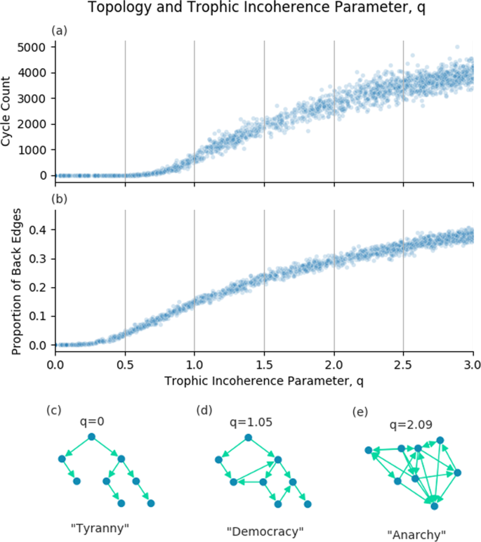
The trophic incoherence parameter’s relation to topological structures. (a) and (b) Show counts of cycles of length 5 and the proportion of back edges in graphs generated using the general Preferential Preying Model with 100 nodes, 750 edges and 5 basal nodes, over a range of the trophic incoherence parameter. At low q (c), graphs are tree-like, analogous to a tyrannical social system. At high q (e), graphs are random with little coherent structure, analogous to anarchy. At mid q (d), there is some coherence, analogous to democracy.

Full size image

Figure 1 shows relationships between the trophic incoherence parameter and topological structures. Johnson et al. showed a theoretical relationship between cycles and trophic coherence²⁶, which suggested that graphs in the low q regime will have very few cycles, this is demonstrated empirically in 1(a). A discussion of how the number of cycles in a graph was calculated is included in the Supplementary Information.

A “back edge” is a link from a node of higher trophic level to a node of lower trophic level i.e. the trophic difference of this edge will be below zero. As described above, we know that the mean of the trophic differences of edges will be 1 for any graph, and that the trophic incoherence parameter is the standard deviation of the distribution of trophic differences. The probability of an edge having trophic difference below zero should therefore increase with the trophic incoherence parameter, q. Figure 1(b) shows that, empirically, the expected number of back edges appears to be an increasing function of the trophic incoherence parameter, q, as expected.

The empirical number of cycles and back edges support our conceptual view of trophic coherence. This gives us 3 regimes of structure, each of which has a social analogus:

1. 1.

   Low q regime. Hierarchical, tree-like graphs with few cycles or back edges. The social analogue is Tyranny.

2. 2.

   Medium q regime. Broadly hierarchical, but with increasing numbers of cycles and back edges. The social analogue is Democracy.

3. 3.

   High q regime. Little hierarchical structure, lots of cycles and back edges. The social analogue is Anarchy.

For our purposes, trophic coherence is a useful concept to describe different types of social systems, and in particular how coherent a social structure is. The trophic incoherence parameter, q, gives us a one-dimensional measure of the slightly abstract concept of coherence, which will allow us to investigate the structure of social systems in a novel and quantitative way.

Network generation model

One of the earliest and most influential random graph generation models is the Erdős-Rényi model³². The Erdős-Rényi graph generating algorithm with node count S and edge count L uniformly randomly places L directed edges across all possible edges between nodes³³. The ensemble includes all possible configurations of ({mathscr{G}}=(V,E)) with those node and edge counts³³. However, Erdős-Rényi graphs have a very low probability of having high trophic coherence. While it is theoretically possible to investigate the entire state space with Erdős-Rényi graphs, we seek a more reliable way of tuning random graphs with specific trophic incoherence parameters, q.

The niche and cascade models arose from the literature on ecology, as attempts to generate artificial food webs similar to empirical food webs using simple rules¹¹. These models generate directed graphs with trophic incoherence parameters in the range 0.5 ⪅ q ⪅ 2. However, we need to generate graphs with a wider range of trophic coherence.

Johnson et al.’s 2014 paper, which introduced the trophic incoherence parameter, q, also introduced the Preferential Preying Model¹¹. This was updated in 2016 as the general Preferential Preying Model²¹, which we will use as our main graph generating model. The Preferential Preying Model was inspired by considering how ecological food webs form in nature²⁹, and it has the advantage of generating graphs over a controllable range of trophic coherence. We will use this graph generation model during our investigation.

The general Preferential Preying Model algorithm requires an input of the number of nodes, S, the number of basal nodes, B, the number of links, L and a Temperature parameter, T, which is used to tune the trophic incoherence parameter of the resulting graph²¹. The algorithm proceeds in 2 phases.

The algorithm begins with B basal nodes, which are given a temporary trophic level, ({hat{s}}_{i}=1). Each of the remaining S − B nodes are added one at a time, with an edge created to the new node, j, from an existing node, i, which is chosen uniformly randomly. The temporary trophic level of the new node is set to ({hat{s}}_{j}={hat{s}}_{i}+1). Once all nodes are added we have a graph with S nodes and (S − B) edges²¹. In phase two, L − (S − B) more links are added, the relative probability of a link being added from node i to node j is given by:

The general Preferential Preying Model generates graphs from a particular ensemble²⁶. Real social systems may exist outside of this ensemble, and may have dynamic structures that change over time. It may be that there is some hidden feature of graphs generated using the general Preferential Preying Model which is responsible for any results or conclusions we find. We will consider graphs generated using the general Preferential Preying Model as a null model, and be wary of over generalising our results to all social systems.

Opinion dynamics

The majority rule model²³ allows each node to be in one of two states, which we will denote as state −1 or state 1, x_i∈ {−1, 1}. We define the state vector as the state of all S nodes, x = [x₁, x₂, …, x_n]. We consider nodes being influenced along the directed edges, with the state of a node changing based on some form of influence dynamics. Considering discrete timesteps, the state of nodes in a timestep are determined by some function on the graph topology and the state of the nodes in the previous timestep²³.

We will use a simple majority rule algorithm to update the states of the nodes at each timestep. At each timestep, t, a node is uniformly randomly selected and its state is updated based on the state of its parent nodes, where a directed link goes from a parent to a child node. The algorithm will update a node’s state to match the state of the majority of its parent nodes in the previous timestep²³. If there is a tie then the node’s state will be determined by a coin flip, with a 50% probability of state −1 or 1²³.

Source: Ecology - nature.com