Pelagic fish predation is stronger at temperate latitudes than near the equator

Data and filtering

We quantified the relative predation that is exerted by large pelagic fish predators based on four publicly available datasets from pelagic longline fishing (West Pacific, East Pacific, Atlantic, and Indian Ocean), each managed by an independent commission (see Supplementary Table 1 for details). All datasets included catch per effort records per month and year at spatial resolutions of 1° × 1° or 5° × 5° latitudinal grids (a small percentage of records reported at lower resolution were removed). For consistency, we aggregated data presented at 1° × 1° resolution to the lower resolution by assigning records to the nearest geographic midpoint of an overlaid 5° × 5° grid. Data availability was limited prior to 1960, and we thus considered only records from 1960 onward (up to 2014 to permit 5-year blocking of the data; see below).

We filtered our datasets in several ways. We filtered out catch per effort records from longlines that were set to catch a specific target species. We also removed incomplete records (when either catch or effort was not reported), as well as suspect entries for which (i) the total number of predators caught was greater than the actual number of hooks set; (ii) the number of hooks set or the number predators caught was not a whole number; or (iii) the number of predators caught was recorded as zero (zero catches are highly unlikely given the many thousands of baited hooks that are deployed into the ocean on each longline; records with zero catches represented no more than 2% of the data in any ocean basin). After filtering (and later removing of extreme [outlier] values, see below), we obtained a total of 359,584 catch per effort records from the 55-year period between 1960 and 2014 across all ocean basins (Supplementary Table 2). The maximal latitudinal range covered by the data was 50°S to 60°N (Supplementary Table 2). We consider the tropics to be the region between latitudes 23.5°S and 23.5°N.

Quantifying predation

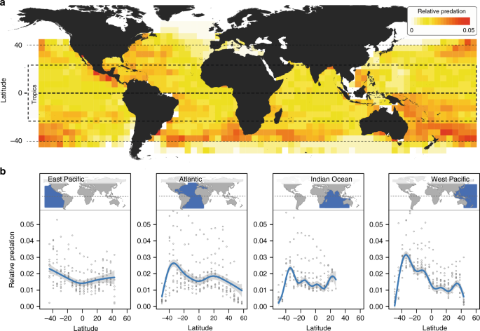
We estimated annual relative predation for each grid cell as the total number of fish predators caught in a year divided by the total number of hooks set that year (akin to a nominal estimate of catch-per-unit-effort, CPUE). This way of measuring predation experienced by a prey organism placed into the wild follows the logic of previous experimental tests assessing predation strength (e.g., refs. ^17,30; see ref. ⁵² for a review). We note that there has been some debate on biases in such tethering experiments, where prey do not have an ability to escape^53,54, potentially leading to an overestimation of predation⁵⁴. However, the size and scope of our datasets may buffer against some of these potential biases, and an overestimation of predation is unlikely to explain relative differences in predation strength across locations to which the same methodology was applied.

Our study is focused on quantifying predation exerted by a large number of open-ocean predatory fish species including tuna, billfish, and shark species (see Supplementary Table 3), but it does not quantify predation by non-pelagic fish predators or by non-fish predators. Acknowledging that we therefore do not quantify total oceanic predation, we refer to the metric of predation used as relative predation. Importantly, however, pelagic fish dominate the predator community between latitudes of about 40°S to 40°N³⁹, which encompasses the majority of our study area. Thus our results are expected to represent a large percentage of the total predation experienced in the study area.

Patterns of variation in predation

We analyzed the relationship between latitude and relative predation separately for each ocean basin using generalized additive mixed-effect models (GAMMs). We used GAMMs because these models infer the simplest function describing variation in relative predation across latitude without making any a priori assumptions about the form of this relationship (e.g., linear, quadratic, etc.). We accounted for spatial autocorrelation in the data by including a spherical data correlation structure term in the model⁵⁵. The latitude and longitude of each grid cell were re-projected to ocean-specific equidistant projections prior to calculating the correlation structure. To reduce possible effects of temporal autocorrelation in our data, we calculated median annual relative predation per grid cell within 5-year time intervals, rather than relying on annual estimates. In addition to ‘latitude’, we included ‘time interval’ as a fixed effect to examine and control for changes in overall relative predation through time. ‘Grid cell’ was included as a random variable to account for the repeated nature of the data. GAMMs were conducted using thin plate regression splines (specified by bs = ‘tp’ in the model syntax, see below) as implemented in the mgcv⁵⁶R-package. The final GAMM syntax was

gamm(attack.rate ~ s(latitude, bs = “tp”) + s(time interval, bs = “tp”), random = list(GridID = ~1), correlation = corSpher(form = ~ latitude_ed + longitude_ed), data = data).

Robustness checks and accounting for methodological variation

We tested the robustness of the overall latitudinal pattern of relative predation against the influence of several potential confounding factors.

Seasonality in fishing pressure: We tested whether seasonality in fishing pressure varied systematically across latitude, potentially biasing the data. We re-ran our ocean-specific GAMMs accounting for the partial effect of season on relative predation, by adding ‘month’ as an additional fixed effect (along with ‘latitude’ and ‘time interval’) into the models. While we do see some evidence of seasonal variation in fishing pressure (Supplementary Fig. 5) and in the latitudinal pattern of relative predation (Supplementary Fig. 6), this variation does not influence our main finding of stronger relative predation away from the equator (Supplementary Figs. 4 and 6).

Number of predatory fish taxa reported and targeted by longline fisheries: We evaluated whether the number of reported fish predator taxa was higher at those latitudes where relative predation was strongest (Supplementary Fig. 7; note that we use the terminology of predator ‘taxon’ instead of ‘species’ throughout this study because longline fisheries catches are not always provided per predator species, but are sometimes aggregated for a group of related fish predator species; see Supplementary Table 3 for details). We then tested whether the bias of fisheries towards certain target species (such as Bigeye or Albacore tuna)—thus resulting in an underrepresentation of non-targeted species—affects latitudinal patterns of relative fish predation based on longline data. Although we could not fully account for missing predators, we asked whether the latitudinal patterns observed for fish predators that are not major targets of longline fisheries are consistent with the patterns observed based on the full datasets. Specifically, we re-ran the GAMMs using estimates of relative predation based only on predator taxa that were deemed ‘non-target’ fish of pelagic longline fisheries (i.e., taxa making up <10% of the total catch within each ocean; Supplementary Table 3). Although temperate peaks in relative predation are weaker in this analysis, we still fail to find evidence to suggest that relative predation is strongest at the equator (Supplementary Fig. 8). Finally, we determined the latitude with the strongest predation per fish predator taxon based on latitudinal means of annual total catch of every fish predator taxon, divided by the total effort per grid cell. Despite marked taxon-specific variation in the strength of predation across latitude, most predation peaks fall away from the equator (Fig. 3 and Supplementary Fig. 9; latitudinal predation patterns for every taxon are depicted in Supplementary Figs. 10 and 11).

Saturation of hooks and heterogeneity in sampling effort: We investigated whether observed patterns of relative predation across latitude could be biased by hook saturation, whereby an increasing number of hooks set would lead to diminishing catch returns. This effect might be exacerbated by removal of fish predators by the fishery itself over time, resulting in lower estimates of relative predation where the number of hooks set (effort) has been excessive. We tested for a saturating relationship between catch and effort in each grid cell within consecutive time periods of 11 years (i.e., 1960–1970, 1971–1981, etc.) using the 359,584 individual catch per effort data records (Supplementary Table 2). Focusing on 11-year time periods provided sufficient individual data records per grid cell to test for hook saturation. Specifically, for each geographic grid cell and time period with at least 20 individual data records, we fitted the exponential function:

where y represents catch and x represents effort (number of hooks). We then took the logarithm of both sides of the formula to fit the linear model:

A value of b less than one should thus indicate hook saturation in a given location and time period. We used GAMMs to determine the extent to which b varies with latitude. Separate models were run for each ocean basin, with ‘latitude’ as a fixed effect, ‘grid cell’ as a random effect, and a correlation term accounting for spatial autocorrelation (akin to the GAMM syntax described in the previous section). Because models including ‘time period’ as a fixed effect did not converge, we accounted for the effect of time by standardizing each slope value by the mean slope across all grid cells from the respective time period. We found that the majority of estimates of b were above 1 rather than below or equal to 1, indicating higher catch per effort with increasing effort rather than saturation (Supplementary Fig. 12A). We lack an explanation for this trend. However, critically, b did not vary greatly with latitude, and consequently did not show the latitudinal variation observed in relative predation (compare Supplementary Fig. 12B with Fig. 1b). Moreover, there was either no or a weak but inconsistent association between total effort and relative predation across latitude in the oceans (Supplementary Fig. 13). The overall pattern of relative predation across latitude is therefore unlikely to be explained by saturation and differences in fishing efforts.

Potential errors in data reporting: GAMMs may be sensitive to extreme values, so we ran GAMMs both with and without values of relative predation that were deemed high or low outliers. Because predation strength was expected to vary by latitude and time, outlier values were identified separately for each latitude in 5-year time intervals based on the individual catch per effort data prior to annual pooling. A value was considered an outlier if it was above or below four standard deviations of the median relative predation within a given latitude–time interval subset. Outlier values represented no more than 2% of the data in any dataset and their removal did not qualitatively affect the results (Supplementary Fig. 14). Our study generally reports results based on datasets with outlier values removed.

Spatial variation in addition to latitude: We re-evaluated the latitudinal pattern of relative predation while accounting for a possible influence of other geographical variables—including longitude, ocean depth, and distance to land—on relative predation. Although some additional variation of relative predation is explained by these variables, the main latitudinal pattern of relative predation remains unchanged (Supplementary Fig. 15).

Further methodological details on all robustness checks are provided as part of the respective figure legends in the Supplementary Material.

Association between latitudinal variation in predation and species richness

We obtained estimates of oceanic fish species richness from AquaMaps⁴⁶. In line with our focus on open-ocean (pelagic) fish predation, we restricted estimates of species richness to “pelagic-oceanic” fish (see FishBase⁵⁷ for classification). Species richness estimates were originally available at 0.5° × 0.5° resolution. To aggregate estimates to the same 5° × 5° resolution used to analyze relative predation, we first consolidated the original records into 1° × 1° grid cells, calculating the mean value for each new cell (four records per cell). We then overlaid our 5° × 5° grid on this grid and assigned species richness to the final grid based on the value at the midpoint of each 5° × 5° cell (where the midpoint of a 5° × 5° grid cell did not correspond to a single estimate of species richness, we averaged across all estimates from the 1° × 1° grid adjacent to the midpoint). To examine the relationship between latitudinal variation in pelagic fish species richness and predation, we calculated median species richness and median annual relative predation for each 5° of latitude from 40°S to 40°N (to account for the effect of time in the overall relative predation [Supplementary Fig. 1], annual relative predation estimates were standardized by the mean value across all cells for that year prior to calculating the median). Spearman’s rank correlation (Rho) was used to quantify the relationship between median species richness and median relative predation for these 5° increments of latitude. We note that the species richness estimated by AquaMaps⁴⁶ is based on range maps, potentially leading to richness overestimates due to errors of commission. However, the latitudinal species richness pattern we observe is likely to be robust to this error because this and related reporting errors are unlikely to vary systematically across latitude.

Reporting summary

Further information on research design is available in the Nature Research Reporting Summary linked to this article.

Source: Ecology - nature.com