Plant diversity effects on forage quality, yield and revenues of semi-natural grasslands

Experimental design

Our study is part of the Jena Experiment, a large-scale and long-term biodiversity-ecosystem functioning experiment in Jena (Thuringia, Germany, 50°55’ N, 11°35’ E, 130 m a.s.l.; mean annual air temperature 9.9 °C, annual precipitation 610 mm; 1980–2010 (ref. ⁶⁶)).

The experimental communities were established in May 2002, covering different plant diversity levels (including 1, 2, 4, 8, 16, and 60 species) and a functional group gradient (including 1, 2, 3, and 4 functional groups) per plot, and were seeded in 82 main plots of a size of 20 × 20 m, adopting a replacement series design. The species pool consists of 60 species typical to Central European Arrhenatherum meadows. Species were categorized into four functional groups, grasses (16 species), small herbs (12), tall herbs (20), and legumes (12) using cluster analysis based on an ecological and morphological trait matrix³². The mixtures were assembled by random selection with replacement, yielding 16 replicates for mixtures with 1, 2, 4, and 8 species, and 14 replicates for the 16-species mixtures. In addition, all 60 species were sown on four plots that were used for comparison in the present study. Plots were arranged in four blocks, regularly weeded to maintain the sown plant diversity levels. No fertilization was carried out in the main plots.

The results presented here are from the Management Experiment setup within the Jena Experiment. For the Management Experiment four subplots of 1.6 × 4 m were established in April 2005 within each of the 20 × 20 m main plots. Each subplot represented one of four additional management intensities with varying fertilization level and cutting frequency per year as listed in Supplementary Table 1 (ref. ¹⁷). The core area of the 20 × 20 m main plots served as one management intensity with two cuts per year and zero fertilizer application (less intensive). The five management intensities ranged from extensive to very highly intensive management, including an extensive management (one cut per year, no fertilization) and a very highly intensive management (four cuts per year, high fertilization of 200 kg N ha⁻¹ a⁻¹ and corresponding P and K fertilization, see below) and three intermediate management intensities: less intensive management (two cuts per year, no fertilization), intensive management (two cuts per year, intermediate fertilization of 100 kg N ha⁻¹ a⁻¹), and highly intensive management (four cuts per year, intermediate fertilization of 100 kg N ha⁻¹ a⁻¹). Thus, the experiment consisted of 390 subplots (82 × 4 management subplots plus 82 core areas). We randomized the allocation of management intensities to subplots, except for the extensive subplots, which were always placed at the plot margins due to logistical constraints. The management intensities selected are representative for common grassland management intensities on floodplains comparable to the experimental site, ranging from grasslands in agri-environmental schemes to intensively managed grasslands¹⁷. We avoided a full factorial design with all fertilization levels per cutting frequency because such a design would include factor combinations that are not reasonable for agricultural practice, such as frequent cutting without fertilization. The controlled manipulation in the experiment of the grassland with different management intensities and different levels of plant diversity, allowed us to test for the presence or absence of a plant diversity effect for different management intensities⁶⁷.

For the preparation of the Management Experiment, we fertilized all four subplots dedicated to the experiment once with 50 kg N ha⁻¹ a⁻¹, 31 kg P₂O₅ ha⁻¹ a⁻¹, 31 kg K₂O ha⁻¹ a⁻¹, and 2.75 kg MgO ha⁻¹ a⁻¹ in April 2005. Starting in 2006, the fertilized subplots received commercial NPK pellets using a lawn fertilizer distributor in amounts presented in Supplementary Table 1. The fertilizer was applied in two equal portions: first in early spring (beginning of April) and second after either the first or second cut (respectively for treatments with two or four cuts) in late June. Plots were cut either once, twice, or four times during the growing season (Supplementary Table 16) with sickle bar mowers at ~3 cm above ground level. All cut material was removed from the plots. Cutting, fertilizing, and weeding were done on a per-block basis such that any maintenance effect was corrected for by the block effect in the statistical analysis.

Data collection and laboratory analysis

We measured biomass yield, and several common and relevant forage quality variables in the harvests of 2007 (Supplementary Table 2)^10,35. Moreover, we estimated contents of metabolizable energy, (metabolically) utilizable crude protein, and milk production potential, all providing valuable information on forage quality related to an agricultural economic perspective.

To measure standing aboveground biomass, we cut all plants within one randomly selected 0.2 × 0.5 m frame in each subplot at 3 cm above ground level, shortly before mowing the rest of a subplot. In the main plots, we cut all plants within four randomly selected 0.2 × 0.5 m frames at 3 cm above ground level. We oven-dried (70 °C, 48 h) and weighed all harvested biomass of sown species. Subsequently, we milled the samples to pass a 1-mm sieve (rotor mill type SM1, RETSCH, Haan, Germany). Dry matter and total ash content were analyzed in these samples by drying at 105 °C and 550 °C, respectively (AOAC index no. 942.05; AOAC, 1997), with a thermogravimetric determinator furnace (TGA 500, LECO Co., St. Joseph, USA). Organic matter was calculated as dry matter minus total ash. Crude protein content was quantified as 6.25 × nitrogen content using a C/N analyzer (Leco-Analysator Typ FP-2000, Leco Instrumente GmbH, Kirchheim, Germany; AOAC index no. 977.02). Following the procedures of Van Soest et al.⁶⁸ using the Fibertec apparatus (Fibertec System M, Tecator, 1020 Hot Extraction, Flawil, Switzerland), we analyzed neutral detergent fiber content, corrected for ash content by addition of sodium sulfite. Contents of ether extract were analyzed with a Soxhlet extractor (Extraktionssystem B-811, Büchi, Flawil, Switzerland; AOAC index no. 963.15). Ether extract content was not reported individually because it is of lower importance as a single variable for forage quality, since it represents only a small share of dry matter, and thus, only of small proportion of energy supply^69,70, but this information was needed for estimating contents of metabolizable and net energy. The content of metabolizable energy was estimated by in vitro fermentation with rumen fluid of a dairy cow, applying the Hohenheim Gas Test procedure⁷¹. In this approach, 200 mg of feed samples were incubated together with 10 mL of rumen fluid and 20 mL of McDougall buffer for 24 h in glass syringes at 39 °C. Afterward, the gas production was measured by a calibrated scale. Together with compositional information, the content of metabolizable energy was calculated by: metabolizable energy (MJ kg⁻¹) = 3.16 + 0.0695 × fermentation gas (mL day⁻¹) + 0.000730 × fermentation gas (mL day⁻¹)² + 0.00732 × crude protein (g kg⁻¹) + 0.02052 × ether extract (g kg⁻¹). Moreover, we estimated the content of net energy for lactation based on the same system, by: net energy (MJ kg⁻¹) = 1.64 + 0.0269 × fermentation gas (mL day⁻¹) + 0.00078 × fermentation gas (mL day⁻¹)² + 0.0051 × crude protein (g kg⁻¹) + 0.01325 × ether extract (g kg⁻¹). We subsequently used net energy for lactation to estimate the milk production potential of the biomass yield⁷². In order to estimate utilizable crude protein content, we collected the mixture of rumen fluid and buffer remaining after incubation of the samples in Falcon tubes and analyzed them for ammonium nitrogen content with the Kjeldahl principle using the distillation unit 323 of Büchi Labortechnik AG (Flawil, Switzerland). Utilizable crude protein content was then calculated by the equation described by Edmunds et al.⁷³ based on analyzed ammonium content in the incubation fluid, obtained with the Hohenheim Gas test procedure without (blank) and with feed (sample), using an ammonia selective electrode (Metrohm AG, Herisau, Switzerland), and the nitrogen content of the biomass yield samples: utilizable crude protein (g kg⁻¹) = [(NH₃-N_blank + N_sample − NH₃-N_sample)/dry matter (mg)] × 6.25 × 1000.

We performed the chemical analyses for the first and the last cut of the year 2007, except for utilizable crude protein content, which we only estimated for the first cut. To retrieve information about the forage quality of harvests from management intensities that included more than two cuts, we used linear interpolation. This was possible, as the forage quality variables showed either a continuous decrease (metabolizable energy content, milk production potential, and crude protein content) or increase (neutral detergent fiber content and ash content) from the first to the last cut. Further, we deleted data from swards that had very small biomass yield or with missing biomass yield information for at least one cut of the year (these were in total 54 swards, from which 31 had a plant diversity level of 1 species, 11 had a plant diversity level of 2 species, 4 had a plant diversity level of 4 species, 7 had a plant diversity level of 8 species, 3 had a plant diversity level of 16 species, and 1 had a plant diversity level of 60 species).

Finally, we calculated the sum of biomass yield of all cuts of a year, i.e., annual biomass yield (g  m⁻² a⁻¹), average forage quality of all cuts of a year, i.e., annual average forage quality (g or MJ or kg kg⁻¹), and the sum of quality-adjusted yield of all cuts of a year, i.e., annual quality-adjusted yield (g or MJ or kg m⁻² a⁻¹):

h includes all cuts of a year.

Analysis of the plant diversity effect

We analyzed the plant diversity effect on biomass yield, forage quality, and quality-adjusted yield using a mixed effect model:

In the Eq. (4), the dependent variable was either annual biomass yield, average annual forage quality or annual quality-adjusted yield. To model the effect of plant diversity, the square root specification (D^0.5) was chosen over others (linear, linear and squared, logarithmic, and D⁻¹), as this specification allowed a diminishing plant diversity effect, which is often observed (see e.g., Hooper et al.⁷⁴), and it performed best across the different outcome variables in terms of the Akaike information criterion and Bayesian information criterion (BIC). More specifically, we modeled the plant diversity effect for each management intensity by introducing an interaction term of the square root of plant diversity and management intensity (D^0.5 × M). Moreover, we included the different management intensities by a dummy variable for each management intensity (M), the interaction term of the presence of legumes with management intensities (L × M), number of functional groups (FG), fixed effects for the presence grasses (G), and tall herbs (H) as well as random effects for blocks (B) and plots (P). Finally, we corrected the results for heteroscedasticity by using robust standard errors. In addition, we conducted a robustness analysis, by using a model with the square root of legume share (number of legumes divided by number of all species) instead of the presence of legumes. This allowed us to account in different ways for the importance of legumes³⁴ and the possibility that the legume share drives the plant diversity effect on nutritive values. Moreover, based on earlier experiments, the Jena Experiment design paid special attention to the role of legumes in grasslands and the interaction with the plant diversity effect, by including legumes in all plant diversity levels, thus avoiding a confounding effect between plant diversity and presence of legumes. However, not every plot included legumes, which offers the possibility to analyze effects of legume presence or abundance³².

We used the Bonferroni correction to correct for perform multiple comparisons (=significance levels/n, n equaled number of different forage qualities, i.e., six, except for biomass yield, for which n was one). Furthermore, we tested whether plant diversity effects per management intensity differed from each other by using a Wald test. To conduct the entire data analyses, we employed Stata 15.0 for Windows.

Economic valuation

To evaluate the on-farm value of plant diversity, we computed the annual revenues of milk sales:

where milk production potential yield refers to the predicted annual mean milk production potential yield per management intensity for different levels of plant diversity. By using milk revenues, we explicitly considered forage quality. The reference price used for the valuation of the milk production potential yield was the average milk price of 2016 and 2017 in Germany of 0.31 Euro kg⁻¹ (ref. ⁷⁵). To adapt dimensions of milk production potential yield to more reasonable dimensions from an agricultural economic perspective, we converted the units of milk production potential yield from kg m⁻² a⁻¹ to kg ha⁻¹ a⁻¹. It shall be emphasized that we assume that farmers maximize their utility, leading to economically efficient decisions (sensu economics). To identify the plant diversity effect, we used the same model as described in Eq. (4) and the Welch t-test.

Typical variable fertilizer and cutting costs (including fertilizer, labor, and fuel costs) in Germany were derived from KTBL⁷⁶, aiming to represent costs in agricultural settings. Costs of increasing fertilization level of our management intensities by one (Supplementary Table 1) of 165 Euro ha⁻¹ a⁻¹ were computed by the amount of calcium ammonium nitrate and PK fertilizer required to meet the change in N, P, and K fertilization multiplied with the respective price (100 N ha⁻¹/0.27 N kg⁻¹ × 0.23 Euro kg⁻¹ + max{43.6 P ha⁻¹/0.12 P kg⁻¹, 83 K ha⁻¹/0.24 K kg⁻¹} × 0.22 Euro kg⁻¹). Additionally, when farmers switch from zero fertilization to some fertilization, variable costs for the process of applying fertilizer (including labor and fuel costs) of 9 Euro ha⁻¹ a⁻¹ arise (0.55 h ha⁻¹ × 13 Euro h⁻¹ + 1.9 l ha⁻¹ × 0.75 Euro l⁻¹). We computed costs of increasing cutting frequency by one cut of 77 Euro ha⁻¹ a⁻¹ considering labor costs and fuel costs for cutting, windrowing, and collecting the harvest ((0.67 h ha⁻¹ + 0.53 h ha⁻¹ + 3.56 h ha⁻¹) × 13 Euro h⁻¹ + (4.85 l ha⁻¹ + 3.18 l ha⁻¹ + 12.67 l ha⁻¹) × 0.75 Euro l⁻¹). Furthermore, we included costs of two alternatives for increasing species diversity: reseeding with seed mixtures and fresh hay transfer. The variable costs of reseeding with mixtures comprise two parts, the actual process (reseeding and rolling⁷⁶) and the purchase of the mixture. The process costs (including labor and fuel costs) of 12 Euro ha⁻¹ a⁻¹ are taken from KTBL⁷⁶ for sites 5 km away from the farm ((0.27 h ha⁻¹ + 0.41 h ha⁻¹) × 13 Euro h⁻¹ + (2.08 l ha⁻¹ + 2.46 l ha⁻¹) × 0.75 Euro l⁻¹). For the mixture costs, we collected prices for mixtures from two online retailers (Fig. 7), of which one focuses on highly diverse regional mixtures (highly diverse mixtures; green cycles). We accounted for production cost differences of single seeds between the shops by replicating the mixtures sold at the standard mixture shop (standard mixtures; orange triangles) with seeds of the shop focusing on species-diverse regional mixtures (price-adjusted standard mixtures; green triangles). The species number of the standard and price-adjusted standard mixtures ranges from 1 to 8 and the respective mean (standard deviation) of the prices for reseeding (20 kg ha⁻¹) are 104 (26) and 229 (36) Euro ha⁻¹ a⁻¹. The diverse mixtures include 38–49 species and the mean price (standard deviation) is 1203 (521) Euro ha⁻¹ a⁻¹.

Fig. 7: Relationship of seed mixtures prices and number of species in the mixture.

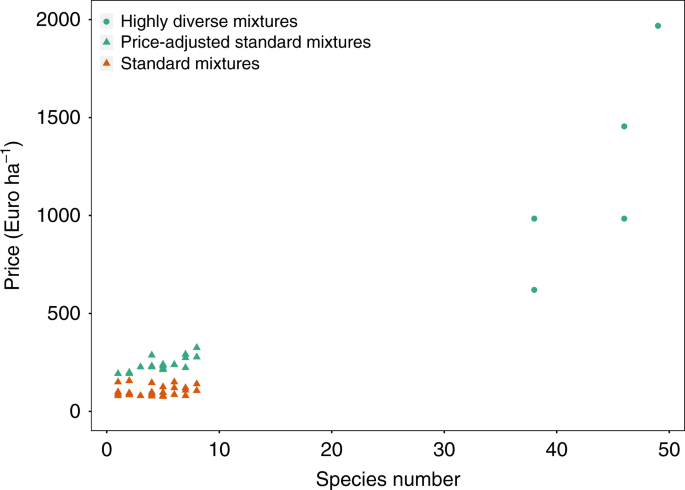
The green cycles are highly diverse mixture (38–49 species). Orange triangles are standard mixtures (1–8 species). Green triangles are price-adjusted standard mixtures, based on seed costs of the shop focusing on highly diverse regional mixtures. Source data are provided as a Source Data file.

Full size image

For deriving reference variable costs for fresh hay transfer, we considered the work steps of cutting, windrowing, collecting, transporting, unloading, and distributing fresh hay^77,78. Moreover, we assumed the use of machinery, a distance of 5 km between the farm and donating and reseeded grassland sites as well as between sites, a hay transfer ratio of 1:1 (ref. ⁷⁸) and no site preparation. We only considered cost for fuel, labor, and opportunity costs, i.e., compensation payment/forgone revenues. The total variable costs of 427 Euro ha⁻¹ a⁻¹ ((0.67 h ha⁻¹ + 0.53 h ha⁻¹ + 5.27 h ha⁻¹ + 3.56 h ha⁻¹ + 0.89 h ha⁻¹) × 13 Euro h⁻¹ + (4.85 l ha⁻¹ + 3.18 l ha⁻¹ + 19.74 l ha⁻¹ + 12.67 l ha⁻¹ + 5.66 l ha⁻¹) × 0.75 Euro l⁻¹ + 250 Euro ha⁻¹) are derived from KTBL⁷⁶ and Kirmer et al.⁷⁷. Note that we always assumed a distance of 5 km between farm and grassland site, and that all costs can change with equipment used, distances, and other factors.

Reporting summary

Further information on research design is available in the Nature Research Reporting Summary linked to this article.

Source: Ecology - nature.com