Progressive nitrogen limitation across the Tibetan alpine permafrost region

Study area

This study was conducted on the Tibetan Plateau, the largest alpine permafrost region around the world, with an area of ~1.35 × 10⁶ km² and a mean elevation over 4000 m^22,23. Climate on this plateau is cold and dry²². The MAAT ranges between −4.1 and 7.4 °C, and the MAP varies from dozens of mm in the northwest of the plateau to ~700 mm in the southeast⁶⁰. Due to the low temperature, permafrost is extensively developed and categorized as continuous, discontinuous, sporadic and isolated types across the plateau²². The mean active layer thickness was estimated at ~2.4 m (range: 1.3~4.6 m) along the Qinghai-Tibetan highway²³. Alpine grassland is the main vegetation type across the Tibetan alpine permafrost region, with dominant species being Stipa purpurea and Carex moorcroftii for alpine steppe and Kobresia pygmaea and Kobresia humilis for alpine meadow⁴⁵. Based on the World Reference Base for Soil Resources classification, the soil type across the study area is dominated by Xerosols and Cambisols⁴⁵.

During the past decade, atmospheric N deposition (Supplementary Figs. 2 and 3), MAP (Supplementary Fig. 2) and soil moisture in the top 10 cm (Supplementary Figs. 11 and 12, and Supplementary Note 3) kept stable across the Tibetan alpine permafrost region. Despite that, MAAT on the plateau has significantly increased with a rate of 0.05 °C per year since 1980⁴⁵, which is similar to the rate reported in the circumpolar permafrost region and twice as much as the global mean warming rate⁴. As air temperature rose, soil temperature was also detected to increase continuously in this alpine permafrost region^23,45. Warming climate has induced extensive permafrost thaw, including top-down permafrost degradation and various thermokarst features, such as thermo-erosion gullies and thermokarst lakes²³. In addition, the Tibetan alpine permafrost region has also experienced a linearly increased atmospheric CO₂ concentration at a rate of 2.2 p.p.m.v. per year (Supplementary Fig. 2). These environmental changes make the Tibetan alpine permafrost region to be a natural laboratory to explore ecosystem N dynamics.

Original and repeated sampling

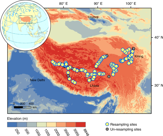
To detect temporal dynamics of ecosystem N cycle in the context of environmental changes across the Tibetan alpine permafrost region, a resampling field investigation, including an original field campaign and a repeated field campaign, was carried out across the study area during 2000s ~ 2010s (Fig. 1). To be specific, the original sampling campaign was conducted by the investigation team from Peking University during the period from 2001 to 2004⁶¹. Based on this original campaign, 135 sites were investigated across the plateau (Fig. 1). After about 10 years, the resampling field campaign was performed by the investigation team from Institute of Botany, Chinese Academy of Sciences in the year 2013 and 2014⁴⁵. With the record of geographic location (latitude and longitude) of a historical site investigated during the 2000s, the resampling site was preliminarily determined by a Global Position System with a decimetre precision (Supplementary Fig. 1a). Based on the soil pits excavated during the 2000s, the resampling site was then accurately located with the help of investigators who participated in the original campaign during the 2000s (Supplementary Fig. 1b). Eventually, 107 (~79%) of the original 135 sites were re-investigated (Fig. 1). These sites spanned about ~3000 km on the Tibetan Plateau, with longitude ranging from 80.8 to 120.1°E and latitude varying between 29.3 and 49.5°N (Fig. 1). Moreover, these resampling sites covered a wide range of climate gradients (MAAT: −3.1 ~ 4.4 °C; MAP: 103 ~ 694 mm) and major vegetation types (59 sites in alpine steppe and 48 sites in alpine meadow) across the study area.

Vegetation samples were collected in the same manner during the two sampling periods. Specifically, in the initial field campaign, a plot of 10 m × 10 m was set up after locating a site and then five quadrats (1 m × 1 m) were established at each corner and the centre of the plot. Within the five quadrats, vegetation communities (occurred species and the relative cover) were investigated and aboveground vegetation was collected for plant δ¹⁵N analysis. In the repeated field survey, once the original 10 m × 10 m plot was recovered (Supplementary Fig. 1b), we set five 1 m × 1 m quadrats next to the original quadrats, investigated vegetation communities (occurred species and the relative cover) and collected all the aboveground vegetation in each of the five quadrats for plant δ¹⁵N analysis (Supplementary Fig. 1c). Consequently, the plant δ¹⁵N measured in our study represented the average isotopic signal of the vegetation community in the five quadrats with 1 × 1 m² area. In other words, the isotopic signal represented information of all the plant species within the vegetation community. Considering the potential effects of shifts in vegetation community on plant δ¹⁵N dynamics observed in this study, we examined changes in vegetation composition indicated by species richness and Shannon–Wiener index (Supplementary Note 1) and detected the stable vegetation community over the detection period (Supplementary Fig. 5). Due to the potential effects of heavily mycorrhizal plant on the community average δ¹⁵N, we further analysed changes in species richness and the relative cover of five families that could be heavily colonized by mycorrhizae on the Tibetan Plateau (Gramineae, Leguminosae, Asteraceae, Cyperaceae and Rosaceae)³³, and examined changes in the relative cover of the dominant species within the five families³³ (Supplementary Note 1). Both the family- and species-level analyses confirmed that vegetation community composition was unchanged over the period from the 2000s to the 2010s (Supplementary Figs. 6 and 7), which eliminated the potential confounding effects of vegetation community shifts on the plant δ¹⁵N dynamics observed in this study.

Similar to vegetation samples, the corresponding approaches used to collect soil samples were also consistent between the two sampling periods. Specifically, soil samples used to measure N isotope, N content as well as other soil properties (texture, pH, soil organic carbon (SOC) content) were collected within the top 10 cm layer in three quadrats along a diagonal within each resampling site (Supplementary Fig. 1c). Soil samples used to determine bulk density were collected within the 10 cm depth with standard 100 cm³ steel cylinders in three quadrats along a diagonal within each resampling site⁴⁵. Besides the identical investigation method and the stable vegetation community (Supplementary Figs. 5–7), the topography and management practices were also unchanged during the detection period for each of the 107 paired sampling sites⁴⁵.

Elemental and stable isotope analyses

To explore changes in ecosystem N cycle, we measured δ¹⁵N values of plant and bulk soil with samples collected through the large-scale resampling investigations. In our study, site-level plant δ¹⁵N measurement was conducted based on the five vegetation samples collected over the five quadrats (1 m × 1 m) within a sampling plot (10 m × 10 m; Supplementary Fig. 1). Specifically, at each sampling site, plant samples were collected from each of the five 1 × 1 m² quadrats, dried to a constant weight at 65 °C and weighed as aboveground biomass separately. The dried plant samples were then ground using a ball mill (Mixer Mill MM 400, Retsch, Germany) for plant δ¹⁵N analysis. In addition, the collected soil samples were air dried, passed through a 2 mm sieve (removing gravel and coarse roots), processed to remove fine roots and ground with a ball mill (Mixer Mill MM 400, Retsch, Germany). With the treated plant and soil samples, we measured plant and bulk soil δ¹⁵N values using an isotope ratio mass spectrometer (SerCon 20–22, Crewe, UK), analysed plant and soil N contents with an elemental analyser (Vario EL Ш, Elementar, Germany), and determined soil P contents with an inductively coupled plasma optical emission spectrometry (ICAP 6300 ICP-OES Spectrometer, Thermo Scientific, USA). To avoid errors in measurements, both δ¹⁵N values and element contents during the two sampling periods were determined at the same time with the same instruments.

Model simulation

To further examine ecosystem N dynamics on the basis of observations from large-scale resampling investigation, we simulated the key ecosystem N cycling processes for the 107 resampling sites with DNDC [http://www.dndc.sr.unh.edu/], a process-based biogeochemical model. DNDC has been widely tested and applied around the world [http://www.globaldndc.net/information/publications-i-3.html], especially for the simulation of ecosystem N dynamics^24,25, and has also been demonstrated to perform well across the Tibetan alpine permafrost region^62,63.

In this study, we first validated the DNDC model in terms of simulating ecosystem-atmosphere nitrous oxide (N₂O) fluxes. Specifically, we collected N₂O fluxes measurements from published studies across the Tibetan alpine permafrost region, and obtained 58 N₂O observations from 22 sites (Supplementary Fig. 15a) in 18 studies (Supplementary Methods). We also synthesized other data from the above-mentioned literature (Supplementary Methods) and other associated literature^64,65,66,67 to drive the model simulation, including vegetation type, plant biomass, plant C:N ratio, soil texture, soil bulk density, soil pH, SOC content and soil C:N ratio. To drive the model simulation, we further acquired data for atmospheric CO₂ concentration, annual rate of atmospheric N deposition, daily meteorology and thermal degree days. Among them, the atmospheric CO₂ concentration, observed at the Waliguan (a global atmospheric background station), was obtained from the Chinese Research Network or Special Environment and Disaster [http://www.crensed.ac.cn]. Atmospheric N deposition rate was obtained from a national-scale spatiotemporal dataset⁶⁸ if it was not provided in the original literature. The daily meteorological data, including mean temperature, maximum temperature, minimum temperature and precipitation, were derived from the nearest meteorological station [http://data.cma.cn/] close to the N₂O observation site. The thermal degree days were calculated by summing the daily mean temperature higher than 0 °C³⁸. Based on the above-mentioned dataset, N₂O fluxes were simulated by the DNDC model. With the simulated and observed N₂O emissions, the model performance was evaluated on the basis of the 1 : 1 line plot (Supplementary Fig. 15b) and four indicators which included R² (coefficient of determination; Eq. 1), RMSE (root mean square error; Eq. 2), RMD (relative mean deviation; Eq. 3) and ME (model efficiency; Eq. 4)^62,63.

where in S_i and O_i are simulated and observed values, (bar S) and (bar O) are their averages and n indicates the number of simulation-observation pairs. The model validation showed that all the data points constituted by the simulated and observed N₂O emissions were well distributed near the 1 : 1 line (Supplementary Fig. 15b), demonstrating good model performance across the study area.

Using the validated model, we conducted simulations for the 107 resampling sites during the period from 1980 to 2015. Before simulations, credible data were collected as model inputs, including atmospheric CO₂ concentration, annual atmospheric N deposition rate, daily meteorological data, vegetation type, plant biomass, plant C : N ratio, soil texture, soil bulk density, soil pH, SOC content and soil C : N ratio. Among them, the annual atmospheric CO₂ concentration, annual atmospheric N deposition rate and daily meteorological data were derived from the Chinese Research Network or Special Environment and Disaster [http://www.crensed.ac.cn], a spatiotemporal dataset of atmospheric N deposition in China⁶⁸ and China Meteorological Administration [http://data.cma.cn/], respectively. The vegetation type for each site was determined based on the vegetation community investigation during the resampling campaign. Data for plant biomass, plant C : N ratio, soil texture, bulk density, pH, SOC content and soil C : N ratio were derived from direct measurements. Of them, plant C content was measured with an elemental analyser (Vario EL Ш, Elementar, Germany). Soil texture was determined with a laser particle size analyser (Malvern Masterizer 2000, Malvern, UK) after removing soil organic matter and carbonate. Soil bulk density was examined by drying the samples collected with standard steel cylinders at 105 °C. Soil pH was determined using a pH electrode (PB-10, Sartorius, Germany) in a 1 : 2.5 soil-to-deionized water mixture. The SOC content was analysed with the Walkley–Black method⁶¹. With the above-mentioned dataset, simulations were conducted with the DNDC model. After that, the model was further validated with the observed soil N density (N storage per area, 0–10 cm, Eq. 5) and aboveground plant N pool (the product of aboveground biomass and the corresponding N content), based on the combination of 1:1 line plots and the four model performance indicators mentioned above (i.e., R², RMSE, RMD and ME). The validation results showed that both soil N density and aboveground plant N pool were well distributed near the 1 : 1 line and the four indicators (i.e., R², RMSE, RMD, and ME) illustrated good model performance (Supplementary Fig. 16).

In Eq. 5, soil N density (SND, kg N m⁻²) was calculated based on soil thickness (T_i, cm), bulk density (BD_i, g cm⁻³), soil total N content (TN_i, g kg⁻¹) and >2 mm rock content (C_i, %)⁵⁵. In addition, soil moisture (10 cm depth) simulated by the DNDC model, determined jointly by precipitation and other hydrological processes⁶⁹, was also validated with the measured values across the 107 resampling sites. The data-model comparison revealed that the DNDC model could well capture the observed soil moisture across the investigated sites (Supplementary Fig. 17). Furthermore, both the simulated and observed surface soil water-filled pore space experienced no significant changes over the period from the 2000s to the 2010s (Supplementary Figs. 11 and 12), demonstrating that the DNDC model could also accurately characterize soil moisture dynamics across the study area.

Statistical analyses

To determine whether N cycling variables exhibited significant differences during the detection period, we conducted statistical tests with the linear mixed-effects model (LMM). LMM is an extension of simple linear model, which can effectively remove the random effects for non-independent data⁴⁵. In this study, LMMs were used to explore changes in plant δ¹⁵N, plant N stress index, the production of available N (soil N mineralization and biological N fixation), plant N demand (plant N pool and plant N uptake rate), ecosystem N loss (total N loss, gaseous N loss and leaching N loss) and bulk soil δ¹⁵N over the detection period. For all the analyses with LMM, the fixed effect was year and the random effect was sampling site. Data normality was tested before the LMM analyses, and log-transformation was performed when necessary. All the analyses were conducted in R 3.5.1 with the lme4 package⁷⁰.

To disentangle effects of environmental changes on N cycling processes, factorial analyses were conducted with the DNDC simulations. Four simulation experiments were carried out for each of the 107 resampling sites: (i) constant atmospheric CO₂ concentration with normal changes in other factors; (ii) constant temperature with normal changes in other factors; (iii) constant precipitation with normal changes in other factors; and (iv) normal changes in all factors. After all the simulations, we calculated the differences between the target variable in one of the four controlling simulation experiments and the target variable in experiment (iv) for each resampling site. Finally, we averaged the calculated differences among the 107 resampling sites to reflect the impact of different environmental changes on the dynamics of N cycling processes.

Source: Ecology - nature.com