Skillful multiyear predictions of ocean acidification in the California Current System

Model simulations

The Community Earth System Model Decadal Prediction Large Ensemble²² (CESM-DPLE) is based on CESM, version 1.1, and uses the same code base, component model configurations (Supplementary Table 2), and historical and projected radiative forcing as that used in its counterpart, the CESM Large Ensemble²⁴ (CESM-LE). This includes historical radiative forcing (with volcanic aerosols) through 2005 and projected radiative forcing (including greenhouse and short-lived gases and aerosols) from 2006 onward. The main difference between the two experiments is that CESM-DPLE is re-initialized annually to generate forecast ensembles (see next paragraph for details), while CESM-LE is only initialized once. We follow the convention of the decadal prediction community²¹ and refer to the former as the initialized ensemble and the latter as the uninitialized ensemble. Because CESM-DPLE and CESM-LE have an identical code base and boundary conditions, the two ensembles can be compared directly to one another to isolate the relative influence of re-initialization and external forcing on hindcast predictability and skill.

CESM-DPLE was generated via full-field initialization each year on 1 November from 1954 to 2017, for a total of 64 initialization dates²¹. An ensemble of 40 forecast members was created by making Gaussian perturbations to the initial atmospheric temperature field (order 10⁻¹⁴ K) at each grid cell. Ensemble spread in all other fields and model components developed as a result of the spread in the atmospheric state. Each member was integrated forward from each initialization for 122 months, resulting in ~26,000 global fully coupled simulation years, costing roughly 50 million core hours to compute. The atmosphere and land components were initialized from the November 1st restart files of a single arbitrary member of CESM-LE (ensemble member 34)³⁶. The atmosphere component is the Community Atmosphere Model, version 5 (CAM5) with a finite-volume dynamical core at nominal 1° resolution and 30 vertical levels^21,37. Details on the land component can be found in Supplementary Table 2.

The ocean (including biogeochemistry) and sea ice model components in CESM-DPLE were re-initialized from the November 1st restart files of a forced ocean-sea ice reconstruction (referred to as the reconstruction; see the following paragraph for configuration details). The ocean biogeochemical model used in all CESM simulations in this study is the Biogeochemical Elemental Cycling (BEC) model, which contains three phytoplankton functional types (diatoms, diazotrophs, and a small calcifying phytoplankton class), explicitly simulates seawater carbonate chemistry, and tracks the cycling of C, N, P, Fe, Si, and O^38,39. Note that the ocean biogeochemistry and simulated atmospheric CO₂ concentration are diagnostic, such that there is no feedback onto the simulated physical climate²¹. Further details on drift adjustment and anomaly generation can be found in the following section.

The reconstruction simulation was run from 1948 to 2017 with active ocean (physics and biogeochemistry) and sea ice model components from CESM, version 1.1, with identical spatial resolutions as the fully coupled CESM-DPLE and CESM-LE (Supplementary Table 2). The ocean and sea ice components were forced by a modified version of the Coordinated Ocean-Ice Reference Experiment (CORE) with interannual forcing^40,41, which provides momentum, freshwater, and buoyancy fluxes between the air–sea and air–ice interfaces. CORE winds were used globally, save for the tropical band (30S–30N), where NOAA Twentieth Century Reanalysis, version 2⁴² winds (from 1948 to 2010) and adjusted Japanese 55-year Reanalysis Project⁴³ winds (through 2017) were used to correct a spurious trend in the zonal equatorial Pacific sea surface temperature (SST) gradient²¹. No direct assimilation of ocean or sea ice observations was used in the reconstruction; thus, any faithful reproduction of ocean and sea ice climatology or variability is due mainly to the atmospheric reanalysis that drives the simulation²¹.

Drift adjustment

Initialized forecasts required drift adjustment due to the use of full-field initialization for the CESM-DPLE. To correct for this model drift, we followed the same procedure as in Yeager et al.²¹. Drift (i.e., lead-time dependent model climatology) was computed as the mean across ensemble members and start dates, separately for each lead time range considered, where only those hindcasts that verify between 1964 and 2014 are included in the climatology. This drift was then subtracted at each grid cell from all forecasts to generate anomalies. Anomalies were computed for CESM-LE and the reconstruction by subtracting the mean over 1964–2014 at each grid cell. The same was done for the JMA observational product, but over the 1990–2005 period that the CESM-DPLE forecasts were verified against. A second-order fit was removed from all time series over their verification window.

Observational product

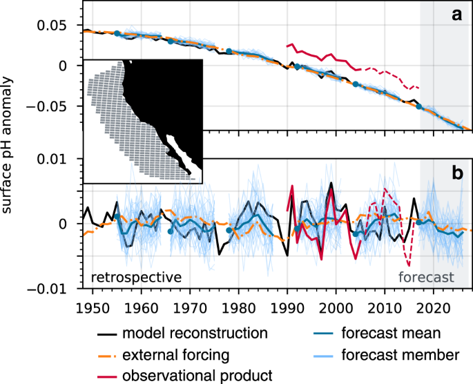
We compare initialized forecasts of surface pH to the Japanese Meteorological Agency (JMA) Ocean CO₂ Map product^25,26, which provides monthly estimates of surface pH from 1990 to 2017 over a 1° × 1° global grid. Here, we describe the key steps followed by the authors of the JMA product to derive their surface pH estimates. Surface pH was computed diagnostically with a carbonate system solver, using estimated surface alkalinity and pCO₂ as inputs. To compute gridded alkalinity, the ocean was divided into five regions, where empirical relationships were derived for in situ alkalinity as a function of sea surface height (SSH) and sea surface salinity²⁵ (SSS). Gridded observations of SSH and SSS (independent of the in situ observations) were then input into the empirical equations to derive gridded surface alkalinity. Gridded surface pCO₂ was computed through a multistep process. First, the ocean was divided into 44 regions and relationships between in situ pCO₂ and in situ SST, SSS, and Chl-a were derived by multiple linear regressions in each region for one to three of the variables²⁶. The gridded pCO₂ product was then derived by applying these functions to independent gridded observations of SST, SSS, and Chl-a. There are no uncertainty estimates available for the pH product, but the authors report a root mean square error (gridded estimate compared to in situ observations) of 10–20 μatm for pCO₂ in the northern hemisphere mid-latitudes and 8.1 μmol kg⁻¹ for surface alkalinity relative to the PACIFICA campaign^25,26. Note that the global average JMA surface pH is within the uncertainty of the SOCAT-based estimate for all years (Supplementary Fig. 9). Further details on the datasets used in deriving their product can be found in Takatani et al.²⁵ and Iida et al.²⁶.

Statistical analysis

We use deterministic metrics to compare the ensemble mean retrospective forecasts to a persistence forecast, and in some cases, the uninitialized CESM-LE ensemble mean forecast. A comparison of the initialized forecast to the persistence forecast shows the utility of our initialized forecasting system over a simple, low-cost forecasting method; a comparison of the initialized forecast to the uninitialized forecast shows the utility of initializations (rather than external forcing) in lending predictability to the variable of interest. The persistence forecast assumes that anomalies from each initialization year persist into all following lead years (or months)⁴⁴. The uninitialized forecast compares the CESM-LE ensemble mean anomalies to the verification data (model reconstruction or observations) over the same window as the initialized forecasting system²¹. Unless otherwise noted, forecasts are analyzed at annual resolution. This corresponds to the January–December average following the 1 November initialization. In turn, lead year 1 truly covers lead months 3–14. When considering monthly predictions, lead month one corresponds to the 1–30 November average following initialization.

We compute the anomaly correlation coefficient (ACC) via a Pearson product-moment correlation to quantify the linear association between predicted and target anomalies (where the target is either the model reconstruction or the observational product). If the predictions perfectly match the sign and phase of the anomalies, the ACC has a maximum value of 1. If they are exactly out of phase, it has a minimum value of −1. The ACC is a function of lead time^10,45:

Where F′ is the forecast anomaly, O′ is the verification field anomaly, and the ACC is calculated over the initializations spanning 1954–2017 (N = 64) relative to the reconstruction and CESM-LE, and over initializations covering 1990–2005 (N = 16) relative to the JMA observational product. We quantify statistical significance in the ACC using a t test at the 95% confidence level with the null hypothesis that the two time series being compared are uncorrelated. We follow the methodology of Bretherton et al.⁴⁶, using the effective sample size in t tests to account for autocorrelation in the two time series being correlated:

Where N is the true sample size and (rho _1) and (rho _2) are the lag 1 autocorrelation coefficients for the forecast and verification data. We assess statistical significance between two ACCs (e.g., between that of the initialized forecast and a simple persistence forecast for the same lead time) using a z test at the 95% confidence level with the null hypothesis that the two correlation coefficients are not different.

To quantify the magnitude of forecast error, or the accuracy in our forecasts, we use the normalized mean absolute error⁴⁵ (NMAE), which is the MAE normalized by the interannual standard deviation of the verification data. The NMAE is 0 for perfect forecasts, <1 when the forecast error falls within the variability of the verification data, and increases as the forecast error surpasses the variability of the verification data. MAE is used instead of bias metrics such as the root mean square error (RMSE), as it is a more accurate assessment of bias in climate simulations⁴⁷.

Where N is the number of initializations and (sigma _{O{prime}}) is the standard deviation of the verification data over the verification window.

Linear decompositions

We follow Lovenduski et al.¹⁷ to convert predictability in pH driver variables (SST, SSS, sDIC, and sALK) to common pH units:

Where r_x is the ACC between anomalies in driver variable x and target anomalies, ({textstyle{{d{mathrm{pH}}} over {dx}}}) is the linear sensitivity of pH to the driver variable, and (sigma _x) is the standard deviation of driver variable anomalies in the reconstruction.

We use a linear Taylor expansion to quantify the relative contribution of variability in environmental drivers to total surface pH variability in the CCS^28,48:

Where primes denote annual average anomalies after removing a second-order polynomial fit, and ({textstyle{{{mathrm{d}}{mathrm{pH}}} over {{mathrm{d}}x}}}) the linear sensitivity of pH to the driver variable x. Residual variability is due to freshwater dilution effects, higher-order terms excluded in the linear expansion, and cross-derivative terms²⁸. Sensitivities were computed using the carbonate system solver, CO2SYS. For example, ({textstyle{{{mathrm{d}}{mathrm{pH}}} over {{mathrm{d}}T}}}) was computed by varying SST by its seasonal range in the CCS in the model reconstruction while holding DIC, alkalinity, and salinity constant at their mean values in the CCS. A linear slope was then fit to the resulting change in surface pH over this range.

Source: Ecology - nature.com