Experimental setup
The experiment was conducted at the experimental dairy farm facility of the Volcani Center, Agricultural Research Organization (ARO), Israel, and was approved by the local ethics committee of the Volcani Center (approval number 412/12IL and 566/15IL).
Animal handling and sample collection: Calves (Holstein-Friesian breed) were divided into two groups: those born by C-section (n = 18) and those born by vaginal delivery (n = 27). Caesarean section is a routine practice for specific breeds of cows63, nevertheless, it is not a common practice among most dairy cow breeds. However, in the context of our study, this procedure was used as a disturbance of the colonizing communities created early in life, which enabled us to ask whether it could affect microbiome assembly dynamics throughout the experimental period.
Animals were subjected to conventional housing and growth practices in our experimental facility. Briefly, calves were immediately separated from their mothers after calving to prevent vertical transmission of microbes from the mother’s oral microbiome to their infants. Calves were housed in individual kennels for 90 days. Thereafter, all animals were housed together in corrals. After 90 days, they were transferred to cohabitation groups. These groups were separated according to their diet, age, and sex. Animals were consecutively transferred from one dietary/age group to the next, in order to keep the different groups as homogeneous as possible. Animal metadata, including sex, date of birth, and mode of delivery, are provided in Supplementary Data 5. The overall cohort, 19 males (males were not castrated) and 26 females, was divided into two groups, C-section-delivered calves (n = 18) and vaginally delivered calves (n = 27). Males were removed from the herd between the ages of 6 and 8 months. Females were sampled for a period spanning 8–28 months. Metadata regarding sample collection can be found in Supplementary Data 6. Females underwent artificial insemination around the age of 480 days and gave birth at around 725 days. Overall, we collected 1634 samples, 1062 samples from vaginally delivered cows, and 573 samples from C-section delivered cows.
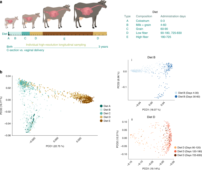
Dietary regime: Calves were fed solely colostrum for the first 3 days after calving. From day 4 until 2 months of age (60 days), calves were fed milk replacer and starter mixture ad libitum. After 60 days, calves were weaned and fed only starter mixture until 90 days of age. From day 90 to 180, calves received a low-fiber diet. From day 180 to ~725 days, animals were fed a high-fiber diet. After calving, a low-fiber diet similar to that supplied between 90 and 180 days was provided. All dietary information is supplied in Supplementary Data 7.
Sampling regime: Rumen sampling was carried out using a custom-made stomach tube (Metal Systems, Kiryat Gat, Israel), which was specifically designed for this study with a length of 2500 mm and diameter of 12 mm. This stomach tube was used throughout the entire experiment for all animals. The design of diameter and length of the tube was based on the physiology of pre-ruminant animals and aimed to reach the ventral part of the rumen from birth to adulthood. The manufacturing of the tube included electropolishing, which minimized injuring the esophagus. The sampling protocol was similar to that of Jami et al.18 and Shabat et al.14, where in younger calves the inserted length of the tube for rumen sampling was based on our initial calibration experiments. In each sampling, the stomach tube was connected to a vacuum pump only when it reached the ventral part of the rumen.
After birth, rumen fluid samples were taken from the newborn calves daily, from day 0 to day 7, due to a previous study in our laboratory that revealed a rapid dynamic changes in microbial composition immediately after birth18. Rumen content was sampled twice more between days 7 and 15. After that, rumen content was collected weekly until weaning. Upon weaning on day 60, rumen fluid was collected weekly until at least 220 days of age, after which samples were collected once a month. Experimental setup and dietary regimes are shown in Fig. 1a. Sampling regime for each individual can be found in Supplementary Data 6 and Fig. S2.
Delivery by C-section: C-section was performed according to the protocol approved by the Animal Policy and Welfare Committee of the ARO. Anesthesia was administered to the mothers paravertebrally using lidocaine and adrenaline. The mother was shaved locally, scrubbed with povidone–iodine solution and washed with isopropanol; the C-section was performed using the left-flank laparotomy approach. The mother was then given penicillin and aminoglycosidic antibiotic and recovery was followed until involution of the uterus.
Bacterial extraction
Thawed rumen samples were transferred to centrifuge bottles and kept on ice for no more than 20 min before processing. Rumen samples were processed as described previously64. The samples were centrifuged at 10,000 × g and the pellet was dissolved in extraction buffer [100 mM Tris-HCl, 10 mM ethylenediaminetetraacetic acid (EDTA), 3% w/v Tween 80, 0.15 M NaCl, pH 8.0]; 1 g of pellet was dissolved in 4 ml of buffer and incubated at 4 °C for 1 h, as chilling has been shown to maximize the release of particle-associated bacteria from ruminal contents65. The suspension was then centrifuged at 500 × g for 15 min at 4 °C to remove ruptured plant particles while keeping the bacterial cells in suspension. The supernatant was then passed through four layers of cheesecloth, centrifuged (10,000 × g, 25 min, 4 °C) and the pellets were kept at −20 °C until DNA extraction.
DNA extraction
DNA extraction was performed as previously described64. Briefly, cells were lysed by bead disruption with phenol followed by phenol/chloroform DNA extraction. The final supernatant was precipitated with 0.6 volume of isopropanol and resuspended overnight in 50–100 μl TE (10 mM Tris-HCl, 1 mM EDTA), then stored at −20 °C.
Animal genotyping
Genomic DNA extracts from 36 animals were loaded into a bovine SNP 50 K chip, which is targeted at 54,609 common SNPs that are evenly spaced along the bovine genome (Illumina). The SNP chip model used was Illumina bovine SNP50-24 v3.0, catalog no. 20000766, and it was processed according to the manufacturer’s protocol at the Genomics Center of the Biomedical Core Facility, Technion, Israel.
Genotype data quality control
QC was performed with the PLINK66 program, with the following parameters: -cow—file isgenotype_all—maf 0.05—geno 0.05—mind 0.05—recode12. SNPs that were not genotyped in more than 5% of the individuals were removed. Similarly, individuals were removed from the analysis if they had been genotyped in less than 95% of the loci (SNPs) covered by the SNP chip. Three individuals were removed because of low genotyping, 3001 SNPs were removed because of “missingness” in the genotyped populations, and 15104 SNPs failed the minor allele frequency (MAF) criteria. The total number of SNPs passing QC was 38359.
Estimating kinship matrix
Cows kinship matrix was built based on autosomal QC-filtered SNP values similarity between cows, by IBS approach using EMMAX67 with command line parameters: emmax-kin-intel64 -v-s-d 10.
16S rRNA gene amplicon sequencing
Sequencing protocols are identical to the earth microbiome protocols see link: http://press.igsb.anl.gov/earthmicrobiome/protocols-and-standards/16s/). Amplification of 16S rRNA gene from the ruminal samples was performed according to Caporaso et al.68 for the V4 region, using the primers 515F (5′-GTGCCAGCMGCCGCGGTAA-3′) and 806R (each reverse primer contained a different 12-bp index, see Supplementary Data 8). The protocol was performed under the following conditions: 94 °C for 15 min, followed by 35 cycles of 94 °C for 45 s, 50 °C for 60 s, and 72 °C for 90 s, and a final elongation step at 72 °C for 10 min. The PCR product (380 bp) was cleaned using the DNA Clean & Concentrator™ kit (Zymo Research) and quantified for fragments containing the Illumina adapters. Sequencing was performed using the Illumina Miseq sequencer. For controls in all our runs, we used non-template controls for each of the samples, and therefore all samples were monitored for contamination (see Supplementary Fig. 21 for representative DNA gel pictures). The product was quantified using a standard curve with serial DNA concentrations (0.1–10 nM). Finally, the samples were diluted to a concentration of 4 nM and prepared for sequencing according to the manufacturer’s instructions. The normalized samples were then unified and sequenced by the paired-end method.
Quality control
Data quality control and analyses were mostly performed using the QIIME 1.9 pipeline68. First, after paired ends were joined, reads were demultiplexed, and read-quality filtering was performed using the default settings of the “split_libraries_fastq” command. Total read count for all 1634 samples was 55,493,183 reads, with an average of 33,270 ± 24,875 reads per sample. All samples were then subsampled to 10,000 reads per sample. The next step was to align the obtained sequences to define OTUs for eventual taxonomy assignment. The Uclust method was used to cluster the reads into OTUs using the pick_otus command at 97% similarity. Taxonomy was assigned using the Ribosomal Database Project (RDP) classifier against the 16S Greengenes reference database (http://blog.qiime.org), designated as ‘most recent Greengenes OTUs’. After an OTU table was created, singletons and doubletons were discarded. The OTU table in biom format can be found in Supplementary Data 9.
Time-point binning
Samples were divided into 58 different time bins according to sampling time; time bins can be viewed in the metadata mapfile (Supplementary Data 6) under the column “time_bins”. Time-point binning was used for α and β diversity over time (Supplementary Figs. 4 and 5) analysis, species arrival rate (Supplementary Fig. 8), and phylum-distribution analysis (Fig. 4a).
Similarity measurement
For similarity measurement between the bacterial communities in the samples, the Bray–Curtis and UniFrac distance similarity indices were used to compare samples according to both presence and absence of OTUs and relative abundance of OTUs between samples. A PCoA eigenvalues table was calculated using the Bray–Curtis similarity matrix. The beta_diversity.py and principal_coordinates.py Qiime scripts were used to calculate beta-diversity indices. Separation of the different samples within diet clusters was performed using PERMANOVA (qiime script: compare_categories.py). Random Forest classifier was applied using qiime supervised learning.py command.
Core successional microbes analysis
Core successional microbes were calculated using compute_core_microbiome.py; the OTU table was collapsed by cow id using collapse_samples.py, and then core successional OTUs were calculated as OTUs present in 80% of all cows. Overall, 2544 core OTUs were found. A core heat map was built using the heatmap.2 command in R. OTU table rows (bacterial species, n = 2544) were clustered using hclust, and columns (rumen samples, n = 1634) were sorted by day of life (see Fig. 3Aii for more details), see Supplementary Data 2 for core microbes OTU table.
Core successional microbes appearance in different dietary regimes
To examine whether bacterial species tend to be diet-specific, we performed a permutation test (n = 100) in which each row was shuffled at each iteration. Thus, the labels comprising each row were changed for each iteration, randomizing time, and diet.
First appearance of core successional microbes vs. all other microbes
A permutation test was performed in which the mean first presence of the core OTUs was measured. Then 2544 OTUs were randomly selected from a list of all other OTUs (core OTUs excluded) and their first presence was averaged. This step was repeated 1000 times.
Species arrival rate
A permutation test was performed in which the arrival of new OTUs into each time bin was measured vs. a null model. The null model was created by random shuffling of the time bin labels. This step was repeated 1000 times. The slope was measured for the non-permuted data using a linear regression model (−74) and averaged across all permutations (−134 ± 0.5).
Persistence analysis
Species persistence was calculated as follows. For each sampling day, we counted the number of species arriving on that day and measured their maximal possible time of appearance within a window of 600 days starting from their day of first appearance (Daylast appearance – Dayfirst appearance). We then averaged the mean time of appearance for each sampling day. This calculation was performed separately on core OTUs and all other OTUs. OTUs appearing later than 430 days of life were discarded due to the lower sampling depth at these time points. We repeated this analysis on OTUs appearing in at least 5, 10, 20, and 30 samples, and received the same results (Supplementary Fig. 9). Nevertheless, we acknowledge the potential confounding effect of ‘low abundant’ molecular species in our analyses, at the level of species that might contribute to the decrease of persistence in the non-core OTUs.
Statistical analysis for persistence of core OTUs vs. all other OTUs was performed as follows: delta (time of last appearance – time of first appearance) was calculated for each OTU, after which sampling days were shuffled and the delta recalculated 100 times. The ratio between real delta and mean permuted delta was calculated. A t-test compared the ratio between core OTUs (0.86) and all other OTUs (0.64) and was found to be significant (P < 0.005, two sided).
Unique species at first time point
To test for a significant association between mode of delivery and species appearance on the first day of sampling, we performed a χ2 test in which the null hypothesis was that there is no relationship between species appearing at time point t = 1 and mode of delivery. We used a contingency table in which we had all species arriving at t = 1 (n = 5067). This table had three columns: the first column was the sum of all species unique to C-section animals (n = 1163), the second was the sum of all shared species (n = 1665), and the third was the sum for all species unique to vaginally delivered animals (Supplementary Data 10). Our test rejected H0, meaning that there is a dependence between mode of delivery and species arriving at time point t = 1 (P < 0.05).
IndVal (delivery mode-associated species)
Because our cohort contained more vaginally delivered than C-section-delivered cows, the first step in performing this analysis was to balance the data. Only 18 vaginally delivered cows were selected, so that the total number of samples from each mode of delivery would be the same. Furthermore, the distribution of the different time points would be as similar as possible. The list of cows selected for each group can be found in Supplementary Data 11.
To determine habitat-associated species (by habitat we refer to C-section or vaginal delivery) among the different communities, we used the R package ‘Labdsv’ and performed the Dufrene–Legendre Indicator Species Analysis (IndVal47,), where x = transposed OTU table, clustering = delivery mode, numiter = 1000. Overall, 1041 OTUs were found to be significant for C-section-delivered cows and 809 OTUs were found significant for vaginally delivered cows (i.e., C-section-associated species and vaginal delivery-associated species, accordingly). A list of IndVal-selected species according to mode of delivery can be found in Supplementary Data 3.
Statistical validation for IndVal-selected species
Since these habitat-associated species accounted for <2% of the overall species cohort, we sought a validation method to determine the significance of these species along the entire sample cohort. We counted the number of habitat-associated species (OTUs) with C-section and vaginal delivery as the differentiating ecological identity and compared this to 100 permutations in which the delivery-mode labels were shuffled (Supplementary Fig. 15).
Phylum-distribution analysis
The distribution of the four main phyla (Actinobacteria, Bacteroidetes, Firmicutes, and Proteobacteria) was calculated by counting the number of OTUs belonging to each of these phyla within each time bin. The difference between the distribution of each phylum between the two modes of delivery was determined by comparing the COM between the two modes of delivery by randomly sampling 70% of the values independently for C-section and vaginal delivery and calculating COM (n = 1000 times). We then compared the two vectors for each phylum (1000 COM values for C-section and 1000 COM values for vaginal delivery) using Wilcoxon test (Supplementary Fig. 17).
The kernel density plot was used to present the distribution of the data (Fig. 3a). Kernel density is a weighting function that quantifies the density of samples and presents them in a smooth manner69. We used the kernel density in order to present a histogram of the density of different phyla along time. Kernel smoothing estimates were applied to each subpopulation (C-section and vaginal delivery) and presented only the four main phyla (Actinobacteria, Bacteroidetes, Firmicutes, and proteobacteria). In Kernel density, Areas with greater point density, in this case higher density of specific phylum, will have higher kernel estimate values at a specific time point, as can be seen in Fig. 3a.
COM
COM is the average time of appearance for an OTU, weighted according to its relative abundance across all sampling points. COM was calculated for each OTU as:
$${mathrm{COM}} = frac{{mathop {sum }nolimits_{i = 1}^n R.A_t cdot {mathrm{Day}}_t}}{{mathop {sum }nolimits_{i = 1}^n {mathrm{Day}}_t}}$$
where i is the cow ID (1–45), R.An is the relative abundance of a species at time point t, Dayt is the day of life when the sample was taken (1–831).
MTV-LMM
MTV-LMM uses a linear mixed model for identifying autoregressive taxa and predictioning their relative abundance at future time points (see Shenhav et al.48 for more details). MTV-LMM is motivated by our assumption that the temporal changes in the relative abundance of taxa j are a time-homogeneous high-order Markov process. MTV-LMM models the transitions of this Markov process by fitting a sequential linear mixed model (LMM) to predict the relative abundance of taxa at a given time point, given the microbial community composition at previous time points. Intuitively, the linear mixed model correlates the similarity between the microbial community composition across different time points with the similarity of the taxa relative abundance at the next time points. MTV-LMM is making use of two types of input data: (1) continuous relative abundance of focal taxa j at previous time points and (2) quantile-binned relative abundance of the rest of the microbial community at previous time points. The output of MTV-LMM is prediction of continuous relative abundance, for each taxon, at future time points.
In order to apply linear mixed models, MTV-LMM generates a temporal kinship matrix, which represents the similarity between every pair of samples across time, where a sample is a normalization of taxa relative abundances at a given time point for a given individual. When predicting the relative abundance of taxa j at time t, the model uses both the global state of the entire microbial community in the last q time points, as well as the relative abundance of taxa j in the previous p time points. The parameters p and q are determined by the user, or can be determined using a cross-validation approach; a more formal description of their role is provided in the Methods. MTV-LMM has the advantage of increased power due to a low number of parameters coupled with an inherent regularization mechanism, similar in essence to the widely used ridge regularization, which provides a natural interpretation of the model.
Training and testing the model
We divide our dataset into three parts: training, validation, and testing, where each part is ~1/3 of the time series (sequentially). We train all four models presented above and use the validation set to select a model for each taxon j, based on the highest correlation with the real relative abundance. Using the validation set, we found p = 1 and q = 1 to be the best model for most taxa and therefore used these parameters. We then compute sequential out-of-sample predictions on the test set with the selected model.
Quality control for sequencing errors
We measured the probability of each OTU in our data set to arise from sequencing errors. Using a method by Jing et al.70 we calculated Poisson probabilities for a single sequence at different similarities for each OTU, considering sequencing error rate of 0.24% as measured for illumina amplicon sequencing71. We defined minor and major OTUs as described in the above method and assessed whether they are artifacts arising from sequencing errors. The probability of each minor OTU arising by sequencing error was determined by multiplying this probability with the number of nucleotides in a given biological sample (which in our case is 250 nucleotides). We next tested for random sequencing error hypothesis for each ‘major’ and ‘minor’ OTUs-species (97% clusters). More than 92% and 94% respectively of the OTUs rejected the null hypothesis (using Benjamini Hochberg multiple hypotheses adjustment). Supplementary Data 12 describes in detail the probability of each minor OTU to represent sequencing errors and Supplementary Data 13 which supplies the OTUs that were not found to be significant after Bonferroni correction.
Finally, we sequenced several technical replicates of several samples in order to detect and calculate the number of spurious OTUs and the error rate. These analyses revealed that the technical replicates are highly similar to each other and contain very low amount of variance compared to biological samples which is mainly due to sampling of rare OTUs as previously described (Supplementary Fig. 20)
We additionaly examined the probability of the non core OTUs presented in Fig. 2b as gray dots (non-core OTUs) to result from sequensing errors. Using the analysis mentioned above we calculated the probability of these OTUs to be the result of sequencing error and found them all to be genuine and to reject the null hypothesis. In addition to this analysis we have measured the robustness of our results by gradually increasing the stringency of our analysis and measuring the validity and robustness of our findings. This analysis resulted in the same conclusions, further strengthening the robustness of these findings. We examined OTUs that appeared in {5, 10, 20, 30} samples (Fig S9) which decrease the probability of these OTUs to be a sequencing error to a maximum of 7.96 × 10⁻¹⁴. This is calculated in the following manner: The error rate per nucleotide that we used is 0.0024 (0.24%). If a given sequence belongs to some focal 97% cluster (let it be cluster A) and was erroneously classified to cluster B, it should have at least eight different nucleotides compared to the OTUs in cluster A. In the most stringent settings, that would be due to an error in one nucleotide, with a probability of 0.0024. Our results show that this stringent analysis did not affect our findings of both core and non-core persistence. With regard to the autoregressive OTUs, we only used OTUs with at least 10% prevalence (appear in at least 160 samples) and for which the probability of being spurious is very low (0.002416).
Quality control by sequencing synthetic communities
In order to test the occurrence of sporius taxa during our clustering and taxonomy assignment processes, we have created triplicates of synthetic consortia composed of 2 and 3, 4, and 5 microbes (See table in Supplementary Fig. S23). We sequenced and analyzed these consortia using the same parameters as described above. Our results accurately identified the species that were introduced into the consortia. Nevertheless, they also show the occurrence of sequence errors that were on average only a negligible fraction (0.0002) of the total relative abundance (Supplementary Fig. 23). We acknowledge the potential confounding effect of ‘low abundant’ molecular species.
Reporting summary
Further information on research design is available in the Nature Research Reporting Summary linked to this article.
Source: Ecology - nature.com
