Sustainability of spatially distributed bacteria-phage systems

A typical set of mass action equations for the bacterial density B, the density of free phages P, and the nutrient n take the form^13,14,23,35:

where the nutrient n is measured in units of bacteria it can be converted to (corresponding to a yield of 1), λ = 2 h⁻¹ is the maximal bacterial growth rate, η = 10⁻⁸ mL/h is the adsorption rate for phages²⁶, β = 100 is the phage burst size, and δ = 0.1 h⁻¹ is the phage decay rate³⁶. K = n(0 h)/5 is the Monod constant³⁷ which determines at which concentration of nutrients the growth rate is halved. The initial nutrient level is set to n(0 h) = 10⁹/mL, meaning there is sufficient nutrient to produce 10⁹ bacteria within a millilitre of medium.

These equations are modified from standard Lotka-Volterra equations by the depletion of food and the associated parameterization of growth by the Monod equation. The above equations are the simplest way to model the development of a bacteria-phage system in a batch culture (e.g. as used for temperate phage dynamics in ref. ³⁵).

Even before considering the effects of space on bacteria-phage interaction, the model noticeably ignores the latency time between phage infection and cell lysis. This is easy to include, either through a time delay equation³⁸ or by introducing some intermediate infected states I_i between infection and lysis^39,40. We choose the latter method and incorporate internal infected states I_i.

The addition of latency time in Eq. 2 is obtained with the use of 10 intermediate infected states (I={sum }_{i=1}^{10}{I}_{i}) between infection and final release of phages⁴⁰. The use of intermediate stages leads to the latency times being drawn from a gamma distribution with an average latency time τ = 0.5 h²⁶ and a variation of 1/(sqrt{10} sim 30 % ) between separate lysis events (see supplement for details). The virulence of phages is dependent on the growth conditions of the bacteria: in nutrient-poor media, the burst size and latency period of the phages are often smaller and longer respectively than in rich media^41,42,43. It is not clear if the measured decrease in burst size is due to fewer infected cells reaching the lysis stage or if fewer phages are produced during the replication stage. In addition, it is well known that most phages cannot grow on stationary phase bacteria, with a few notable exceptions such as T7⁴⁴. In our simulations, the transition from exponential phase to stationary phase is controlled by the amount of nutrient available. Therefore, we scale the latency between infection and lysis by the same Monod-like factor that controls bacterial growth. This means that as the nutrient is depleted, the latency time increases with bacterial generation time and thereby the phage invasion stops as the stationary phase is reached since no progeny phages can be released.

Notice that the addition of infected states reduces the virulence of phages not only by the introduced latency time, but by their mere presence. The phages do not discriminate between infected and uninfected bacteria so the phages also “waste” their genetic material by superinfecting the already infected bacteria. Note that the bacterial density, B, now refers to the uninfected bacteria, not the total bacterial density.

The above model corresponds to liquid conditions where the medium is continuously disturbed, e.g. by shaking. In this situation, the bacteria and phage are well-mixed and freely interact. If however the medium is left standing, then inhomogeneities may amplify and we use the spatiotemporal equation:

The populations (B, P, I₁, …, I₁₀) and the nutrient n are now functions of space (x, y, z) as well as time, but we keep the parameters constant throughout. For readability, we don’t explicitly include the spatial dependency in the notation. In the model, D_n, D_B, and D_P are the diffusion constants for the nutrient, the bacteria, and the phages respectively. Here D_n ~ 10⁶ μm²/h⁴⁵ is much larger than D_P ~ 10⁴ μm²/h^46,47 and D_B ~ 5 ⋅ 10² μm²/h⁴⁸ (assuming no chemotaxis).

With these equations, we now model how delayed lysis and spatial heterogeneity in the population densities moderate the virulence of the phages. This limit corresponds to the situations where the bacteria are not immobilized and thus do not form colonies, e.g. as in standing liquid medium. The spatial heterogeneity then comes from the difference in diffusion rates where bacteria move substantially slower than the phages.

If the medium is more solid, the growth of the bacteria becomes even more spatially structured and submillimetre scale spatial structures related to bacterial colonies emerge. In these structured environments the bacteria are fully immobilized and do not diffuse (D_B = 0). Taken together, we present our full model for phage-bacteria interaction in a spatial context.

The new concepts included in this model are shown schematically in Fig. 1 as a guide to the reader.

We investigate scenarios where the bacteria are constricted in the medium and remain effectively immotile. This situation is for instance encountered when performing experiments in soft agar⁹, but there are several other systems where the bacteria are constrained (such as in soil, biofilm, or solid foods). This constriction in space means that each initial bacteria grow to a colony of size (B + I)/n_c, where n_c(x, y, z) = B(x, y, z, 0 h) is the density of the initial bacteria and thus the density of colonies (see Fig. 1(b)), and I is the density of infected cells.

When bacteria grow in colonies, as opposed to growing separately, the dynamics of phage adsorption changes. Therefore, when a phage is adsorbed to one of the n_c colonies, it does so with a rate that is proportional to the colony radius^33,34 (hence the (frac{1}{3}) exponent, see supplement for more details).

When some bacteria in the colony are already infected, then only a fraction S of the infections leads to new infected states, since the accumulated infected cells exist on the surface of the colony and partially shields the uninfected cell from the phage attack⁹. The remaining fraction 1 − S adsorb to these infected surface cells and consequently “waste” their genetic material to superinfecting bacteria instead of adsorbing to uninfected bacteria. This protection is defined by the shielding function S, which we will explain further below.

When lysis occurs, the released phage has a high probability of reinfecting the colony, which is represented by the parameter α = 0.5. A fraction (1 − α) of the phage progeny escape from the colony and becomes free phages P, while a fraction α readsorbs to bacteria in the colony. The functional form of the readsorption, as well as the value of α, is somewhat arbitrary, since we do not have a good model for what it means to “escape” a colony, nor do we have a model for how many phages should readsorb within a reasonable timescale. Instead, we use α as a simple way to penalize colony growth. In the supplement, we investigate several values of α and find that the survival of the bacteria is largely unchanging for α values between 0.5 and 0.95.

Returning to the choice of shielding function S, we investigated various shielding functions (see supplement for details), and found an approximate shielding function of the form:

The derivation of this shielding function is inspired by particles moving through an absorbing barrier. Here the phages act as the particles and the barrier is the layer of infected cells, which has a thickness of ({r}_{0}left({left(frac{B+I}{{n}_{c}}right)}^{frac{1}{3}}-{left(frac{B}{{n}_{c}}right)}^{frac{1}{3}}right)), where r₀ is the radius of a single bacterium. The parameter ζ is the typical distance that a phage can penetrate before being absorbed (in units of r₀). If the barrier is thinner than ζ, then most phage will pass through the barrier and vice versa. A nice feature of this shielding function is that there always is a non-zero chance of a phage slipping through the barrier. In the supplement, we estimate ζ as a function of the phage adsorption coefficient via detailed simulations of colonies consisting of individual spherical bacteria and find that for the diffusion-limited case ζ is roughly 1.

Note that to match in the shielding in the small colony limit where the probability of hitting an uninfected bacterium is just the fraction of uninfected bacteria in the colony (S(B, I, n_c, ζ)(=frac{B}{B+I})), we must force an upper limit on the shielding:

In our implementation of the model, we use the above partial differential equations (PDEs) as a guide to design a discrete stochastic model on a lattice. The benefit of the stochastic model is that this more closely mimics the discrete nature of the bacteria and phages at the small scale. The solution to the PDEs will unfairly favour phage spreading since fractional infections of single bacteria will allow the phage population to increase earlier than would otherwise be the case. When the local number of bacteria or phages is small, our stochastic simulation include the associated fluctuations of populations between the boxes. When population numbers are persistently large, each process in the above equations occurs many times in each bacterial generation, and self-averaging over many events approximately eliminate any sign of stochastic variation.

We thus go from densities to integer populations and thereby track individual particles in the simulation. The only exception to this is the nutrients which we treat as a continuous field. Note that the use of integer populations allows for clearly defined extinction scenarios since the populations can reach zero members. In contrast, if using continuous densities, we would need to apply some threshold value for the populations to have well-defined extinction events.

We include the spatial variation by simulating a one cubic centimetre system where space is subdivided into a 3-dimensional lattice consisting of boxes of length ℓ = 0.2 mm. This approach allows for different numbers of bacteria and phages in each of the 1.25 ⋅ 10⁵ boxes in the lattice. We initialize the simulation by placing the individual bacteria and phages uniformly in the simulation space. Note that in order to represent the behaviour of a larger system we use periodic boundary conditions.

Inside each box in the lattice, we simulate our model stochastically by treating each term in Eqs. 1–4 as rates corresponding to events. At each time step, we compute the probability for every particle to undergo each event and draw the number of occurrences from a Poisson distribution (see supplement for details). Every box is simulated independently, modulated by diffusion of food and phages between the boxes. We treat each phage as performing a random walk on the lattice and during each time step we migrate appropriate fractions of the phage population to the neighbouring lattice boxes. Nutrient diffusion is computed by using a discrete Laplace operator (using the “forward time central space” scheme).

Since our lattice is resolved at a resolution of ℓ = 200 μm, we can approximate the bacteria as being effectively immotile (D_B = 0) since they diffuse on average  ~ 30 μm per hour and thus would be unlikely to travel much further than to the boxes immediately adjacent in the time frame we simulate. Note that if we were to resolve lattice at a much smaller resolution we would need to account for cell shoving dynamics which would redistribute the local bacteria into neighbouring boxes when the density approaches the capacity of the grid point.

The problem contains two different timescales, that of bacteria and phages versus that of nutrient diffusion, which is the fastest timescale. In order to solve nutrient diffusion accurately we require that ({D}_{n}frac{Delta T}{{ell }^{2}}le frac{1}{6}) (see supplement for derivation), which we obtain for time steps of size ΔT = 2 ⋅ 10⁻³ h ~ 7 s.

In Fig. 2, we show an example of a single simulation. Here the spatial heterogeneity is evident both in the separation of bacteria colonies in the lattice (blue spheres) but also in the distribution of phages (red points). This is most clearly seen by the small “clouds” of phages diffusing away from areas where the invasion has taken hold.

Figure 2

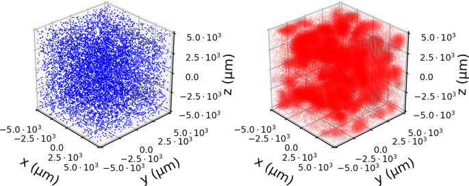
Snapshot of a simulation. The spatial distribution of bacteria (blue) and phages (red) at time T = 7 h starting from an initial B = 10⁴ bacteria per mL and P = 10⁵ phages per mL. To show the variation in densities, we scale the opacity of each point to be proportional to ({rm{log }}10) of the population in that point. Despite uniform initial distributions, the stochastic dynamics cause large variation which is most clearly seen in the patchy distribution of phages.

Full size image

Note that the model we present in Eq. 4 has Eq. 3 as a limiting case: If colonies do not form, then the number of colonies is equal to the number of bacteria (left({n}_{c}=B+Iright)) and the probability of hitting uninfected bacteria is equal to the fraction of uninfected to total bacteria (left(S=frac{B}{B+I}right)). In addition, the phages do not benefit from having adsorbed to the colony so α = 0. Furthermore, the model in Eq. 2 is a limiting case of Eq. 3. The only difference between these models is the inclusion of spatial variation.

The implementation of this model and the data generated by it can be found at the GitHub repository located at https://github.com/RasmusSkytte/SpatialBacteriaPhageModel/tree/v1.03

Source: Ecology - nature.com