Systematic selection between age and household structure for models aimed at emerging epidemic predictions

Aspects common to all models

All models share the same stochastic, time-since-infection transmission process^8,58: each infected individual makes infectious contacts at a rate described by a function βω(τ), where the total infectivity β depends on the ages of the infector and the other contacted person, as well as on the environment (i.e., within or outside the household), and the infectious contact interval distribution ω(τ)⁵⁹ is a function of the time since infection τ, normalised to integrate to 1, with mean T_G (often referred to as the generation time³⁷) and is the same between every pair of individuals, irrespective of age and environment (see Supplementary Methods, Section 1.1.2). After infection, individuals cannot be infected again.

The dynamics of this model, at least in its deterministic form and in the absence of household structure, could be described in terms of a renewal-type integral equation^8,58, with β = R₀, but we do not present it here because no dynamical equations are solved in this work. Instead, for all models, the observables defined during the exponentially growing phase and used for the mapping (i.e., R₀, the incidence ratio of adults and children and the SAR), as well as the final size z, are computed directly using available mathematical results, whereas the peak incidence π and time to the peak t are computed as the average of 100 individual-based stochastic simulations in a population of 100,000 individuals. The epidemics are started with n₀ = 50 initial cases, to avoid stochastic extinction and minimise the effect of random delays at the start of the epidemic, and are synchronised at the peak.

Inspired by influenza, we choose a Γ-shaped infectious contact interval distribution ω(τ) with mean T_G = 2.85 days and shape parameter α = 9^8,32. However, this particular choice does not affect the quantities calculated analytically (observables and final size), which are all time-integrated quantities, and hence bears no influence on the mapping procedure, although it does affect the peak incidence π and the time to the peak t. However, to allow generalisations to other infections, the time to the peak is rescaled by a factor T_G, thus approximately measuring the average number of generations to the peak.

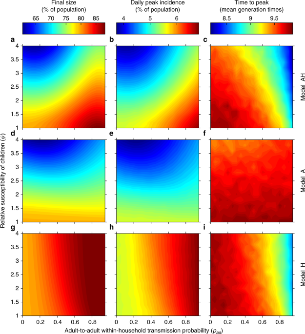
Although the stochastic simulations are computationally intensive, the forward problem of computing observables and outputs for each model is relatively inexpensive even in the absence of analytical results, as it needs to be performed once for each combination of basic model parameters. Instead, the inverse problem of exploring parameter spaces at fixed observables is in general computationally expensive. In the presence of explicit expressions for the observables, which is rarely the case, one could simply invert them to map parameters directly from one model to another⁴². In the absence of explicit expressions, iterative methods must be used (see Supplementary Methods, Section 1.1.1), which require solving the forward problem multiple times and might become prohibitive for computationally costly simulations. The efficiency of our approach stems from the fact that the context we have focussed on, though rather specific, is rich in analytical results: in particular, thanks to the latest methodological advances in the computation of R₀ for households models^47,60, the observables of all models can be obtained without having to integrate the system dynamics. Therefore, the mapping procedure could be performed on all points of a regular grid in the parameter space of model AH (Figs. 1, 2a and 3) that is fine enough to suggest our conclusions, though numerical in nature, hold throughout the explored portion of space.

Model AH (age and households)

Model AH is parameterised as follows. The infection spread between adults (a) and children (c) in each environment x (in the community, x = g for “global”; or in the household, x = h) is parameterised in terms of a next-generation matrix (NGM) of the form

(derivation in Supplementary Methods, Sections 1.1.4 and 1.1.5), where ({k}_{ij}^{x}) gives the average number of infectious contacts an individual in age-class j makes with individuals in age-class i in environment x. In the initial phase of the epidemic all the infectious contacts ({k}_{ij}^{g}) in the community lead to real infections. In a household, instead, some of the ({k}_{ij}^{h}) infectious contacts hit previously infected or immune cases.

The NGM K_x incorporates simultaneously both contact and transmission elements. The contact patterns are given by: γ_x, the ratio of the numbers of daily contacts an adult and a child have in environment x; ({N}_{a}^{x}) and ({N}_{c}^{x}), the numbers of adults and children in environment x, respectively; and θ_x, the assortativity of children in x, defined somewhat non-standardly as the fraction of contacts that a child makes with other children in x and ranging from 0 (fully antiassortative mixing) to 1 (fully assortative mixing). Random mixing is achieved for θ_x equal to the fraction of other children in the environment. Within-household mixing is always assumed to be random (note that this requires θ_h to depend on the household composition). We assume frequency-dependent contact patterns in the households, so that the infectious contacts ({k}_{ij}^{h}) are distributed among all (other) cases of age-class i; that is, in the simple case of all identical individuals, the person-to-person contact rate in a household of size n scales as 1 ∕(n − 1)—see Supplementary Methods, Section 1.2.3, for precise age-stratified details.

The transmission component of the model is parameterised in terms of ψ and ϕ, which represent respectively the relative susceptibility and infectivity of children versus adults, and total infectivities β_x. In practice, the within-household total infectivity β_h is re-parameterised in terms of p_aa, defined as the probability that a randomly selected susceptible would be infected directly by a single initial household case, in a randomly selected household with at least two individuals, when adults and children have the same susceptibility and infectivity (ψ = ϕ = 1). In other words, p_aa is obtained by first computing p_n = 1 − exp(−β_h ∕(n − 1)) and then averaging p_n over the size distribution of a randomly selected household with at least two members. Other similar choices would have been possible, as long as they do not depend on other parameters we are exploring independently, like ψ or ϕ. In the Supplementary Discussion (Sections 2.1.1 and 2.2.1) we comment on more aggregate, but more intuitive epidemiological quantities, such as the SAR or the fraction of total transmission occurring in households. The latter is measured as (left({R}_{0}-{R}_{0}^{g}right)/{R}_{0}), where ({R}_{0}^{g}) is the dominant eigenvalue of K_g, and reveals that, at least for the H1N1 2009 pandemic influenza in Great Britain, approximately a third of the total transmission occurs in household (a rule of thumb suggested before^8,9,32; see Supplementary Discussion, Sections 2.1.1 and 2.2.1).

Numerical values are as follows. At baseline, the population structure is that of Great Britain⁶¹, with a fraction F_c = 22.73% of the population consisting of children and a mean household size χ = 2.35 (see Supplementary Methods, Section 1.6.1, and Supplementary Tables 1–4). Other social structures (South Africa: F_c = 45.92%, χ = 4.27; Sierra Leone: F_c = 53.81%, χ = 5.85) are explored in the Supplementary Methods, Section 1.6.2, Supplementary Tables 4–7 and Supplementary Discussion, Section 2.3.4. At baseline, contact patterns assume random mixing: γ_h = γ_g = 1 (adults and children have the same contact rates everywhere) and θ_g = F_c = 22.73%, the fraction of children in the population. Parameters for UK-like contact patterns, characterised by strongly assortative mixing, are estimated from the POLYMOD study²⁵ to be γ_h = γ_g = 0.75 and θ_g = 58% (see Supplementary Methods, Section 1.6.3, and Supplementary Table 8), and are used also for other social structures (in the absence of contact pattern data for South Africa and Sierra Leone). Intermediate contact patterns are explored in the Supplementary Discussion (Section 2.3.1).

The observables for model AH are derived as follows. The basic reproduction number R₀ is computed using a multitype extension of the technique developed in⁶⁰ that leads to the construction of a suitable matrix M (details in the Supplementary Methods, Section 1.2.4), the dominant eigenvalue of which is R₀.

From M it is also possible to reconstruct the vector ({v}^{{rm{AH}}}={left({v}_{a},{v}_{c}right)}^{top }) (superscript ^⊤ denotes transposition, to give a column vector), whose components are the fractions of adults and children in each generation (v^AH is constant during the exponentially growing phase), correctly computed by taking into account both household and global transmission (Supplementary Methods, Section 1.2.5). Primary cases in households are infected globally, so arise in proportions given by the components of the vector ({v}_{h}^{{rm{AH}}}={left({v}_{h}^{a},{v}_{h}^{c}right)}^{top }), obtained by renormalizing K_gv^AH so that its components sum to 1.

The SAR is defined as the fraction of initial susceptibles that are infected in a within-household outbreak started by a single individual in a typical household infected during the exponentially growing phase. Its computation is not trivial, because the distribution of infected households during the exponentially growing phase is affected by the age-dependent between-household transmission: if children are more likely to be infected in the population, larger households are also more likely to be infected because they tend to contain more children. We denote by (left{{pi }_{n}^{a}right}) and (left{{pi }_{n}^{c}right}) the size distributions of the household of a randomly selected adult and child, respectively, and by μ^a and μ^c the average epidemic sizes in the household of a randomly chosen initial adult or child case, respectively. Then the average size of a household epidemic during the exponentially growing phase is ({mu }^{{rm{AH}}}={v}_{h}^{a}{mu }^{a}+{v}_{h}^{c}{mu }^{c}). The household SAR is then computed as (μ^AH − 1)∕(χ^v − 1), where χ^v is the average size of a household infected in that phase (see Supplementary Methods, Section 1.2.6).

Finally, the outputs for model AH are derived as follows. The average final size z, in the asymptotic limit of an infinite number of households, is computed using the methodology described in ref. ³⁰ (Supplementary Methods, Section 1.2.7). The peak incidence and the time to the peak are obtained from individual-based stochastic simulations in a synthetic population with the required social structure and contact patterns (Supplementary Methods, Sections 1.2.8 and 1.5). To minimise the convergence time from the initial conditions to the stable proportions of cases of each type during the exponentially growing phase, the n₀ initial cases are all chosen as primary cases in different households and consist of adults and children in proportions given by ({v}_{h}^{{rm{AH}}}).

Further details about model AH can be found in the Supplementary Methods, Section 1.2.

Model A (age)

Model A is parameterised as follows. The spread between adults and children in model A is described by K^A, a NGM of the same form as the one in Eq. (1), but with elements indexed by A (there is only one environment). The contact patterns are given by γ^A, the ratio of the overall number of contacts an adult and a child have, and the assortativity of children θ^A. The transmission component of the model is parameterised in terms of an overall transmission parameter β^A and the relative susceptibility and infectivity of children versus adults, ψ and ϕ, which are thought of as biological parameters ideally accurately measured via detailed household studies, and are therefore assumed to be the same as in model AH. The presence of four parameters, two of which coincide by construction with those of model AH, makes model A both more flexible and more tightly linked to model AH than to model H (two parameters only). This partly explains why model A is better than model H at mirroring the outputs of model AH in Fig. 1.

Numerical values are inherited by the social structure and mixing patterns of model AH. At baseline (Great Britain⁶¹) the fraction of children is 22.73% and adults and children have the same contact rate (γ^A = 1). UK-like contact patterns are given by γ^A = 0.75. The assortativity θ^A is estimated in the mapping procedure (see below).

In terms of observables, the basic reproduction number R₀ in model A is computed as the dominant eigenvalue of the NGM K^A, and the corresponding eigenvector v^A, normalised to have components summing to 1, represents the fraction of adults and children in each generation⁵⁸.

In terms of outputs, the final size is computed using standard methods⁵ (Supplementary Methods, Section 1.3). The peak incidence and the time to the peak are again computed using the individual-based stochastic simulation, with no household structure and starting with n₀ initially cases, consisting of adults and children in proportions given by the components of the vector v^A (to start as close as possible to the stable proportions of adults and children during the exponentially growing phase).

Further details about model A can be found in the Supplementary Methods, Section 1.3.

Model H (households)

The pure households model is parameterised in terms of a global total infectivity ({beta }_{g}^{{rm{H}}}) and a within-household total infectivity ({beta }_{h}^{{rm{H}}}), representing, respectively, the average number of infectious contacts an infective makes in the community and in their household, during their entire infection period. Early on in the epidemic, every infectious contact in the community leads to a new infection. Frequency-dependent contact patterns are assumed within the household, so that the number of infectious contacts toward a single member of a household of size n is ({beta }_{h}^{{rm{H}}}/(n-1)).

Numerical values are again inherited by the household structure of model AH. At baseline, the household size distribution is that of Great Britain, with a mean household size χ = 2.35 (see Supplementary Tables 1–3). Other social structures are also considered (South Africa: χ = 4.27; Sierra Leone: χ = 5.85).

The computation of R₀ for model H follows the method of^47,60 (Supplementary Methods, Section 1.4). Similarly to model AH, the SAR is computed as (μ^H − 1)∕(χ − 1), where μ^H is the average size of a within-household epidemic, computed using standard methods for small populations^5,62 and χ is the average household size. However, care needs to be taken in the choice of the correct household size distribution (see below).

The final size is computed using standard analytical techniques²⁸, and the peak incidence and time to the peak are obtained from stochastic simulations starting with n₀ cases, all primary cases in different households, divided in adults and children according to the components of ({v}_{h}^{{rm{AH}}}) (to start as close as possible to the stable household size distribution of the exponentially growing phase).

Further details about model H can be found in the Supplementary Methods, Section 1.4.

Model U (unstructured)

Given the temporal details of the infection process are fixed by the infectious contact interval distribution ω(τ), the model with pure homogeneous mixing has only one parameter β = R₀. The final size is computed standardly as the only positive solution z of (1-z={{rm{e}}}^{-{R}_{0}z}) ⁵, whereas the peak incidence and the time to the peak are obtained via simulations starting with n₀ initial cases.

Model-mapping procedure

For each combination of basic parameters for the assumed-true model AH (ψ, ϕ, p_aa, from which β_h is derived, and β_g—as well as fixed θ_g, γ_g, and γ_h—we calculate the true epidemic observables R₀, v^AH, and SAR, as described above. In practice, the parameter space in all figures is explored at constant R₀, so that for each choice of p_aa, ψ, and ϕ we compute the value of β_g required to achieve a desired R₀. These observables are then used to map the parameters for the other models as follows.

We start by mapping model AH to model A. Parameters ψ and ϕ in model A are assumed to be known and the same as in model AH. Then θ^A is ideally chosen to match v^AH. Unfortunately, there are parameter values for which no suitable value of θ^A∈ [0, 1] can be found (see Supplementary Methods, Section 1.3). This is often the case for ψ < 1 (Supplementary Discussion, Section 2.3.3). The overall infectivity β^A is then chosen to match R₀. There are no households in model A, so the SAR is not used.

To map model AH to model H, first ({beta }_{h}^{{rm{H}}}) is computed to match the observed household SAR. The correct household size distribution to use cannot be computed from model H alone, because the distribution of infected households during the exponentially growing phase is affected by the age-dependent transmission as described for model AH. In real scenarios, the within-household infectivity is measured from household studies. In such surveys, the recruitment of households is subject to many constraints, but it ideally monitors a representative portion of the population of infected households. If model AH were an exact description of reality, then households would be recruited with size distribution (left{{pi }_{n}^{v}right}), where, for each n, ({pi }_{n}^{v}={v}_{h}^{a}{pi }_{n}^{a}+{v}_{h}^{c}{pi }_{n}^{c}). In practice, instead of matching the same SAR as in model AH, we equivalently compute ({beta }_{h}^{{rm{H}}}) by imposing μ^H = μ^AH, with household size distribution (left{{pi }_{n}^{v}right}) (and hence χ = χ^v). The global infectivity ({beta }_{g}^{{rm{H}}}) is then computed to match R₀. Apart from appearing in the computation of the correct household size distribution for matching the SAR (rather than obtaining such a distribution from a random sample of infected households), v^AH is not explicitly used.

Finally, the mapping from model AH to model U is trivial, as model U is only parameterised in terms of R₀ and the other observables are not used.

Reporting summary

Further information on research design is available in the Nature Research Reporting Summary linked to this article.

Source: Ecology - nature.com