The demographic decline of a sea lion population followed multi-decadal sea surface warming

All the analyses described below were based on algebraically explicit Bayesian regression models^52,53, whose parameters of interest were estimated as samples from their posterior distributions through a Markov Chain Monte Carlo procedure, implemented in the language Just Another Gibbs Sampler (JAGS)⁵⁴ in R⁵⁵. This approach avoids the loss of information through the propagation of uncertainty between connected estimations and models, accounting effectively for scarce and/or sparse data, if needed. We ran one million iterations in five independent chains, retaining every 20th value to avoid autocorrelation, and discarding the first 20% as a burn-in phase for each chain (see detailed algebraic explanations and JAGS codes below). The results of the estimations are reported throughout the text as their medians, accompanied by ranges that represent the 95%-credible intervals of the posterior distributions. All the data needed to run the models is provided fully arranged as three R’s data list objects in the Supplementary Information File S1.

Population abundance and trend

When estimating abundance of pinnipeds, pup counts are typically used to infer those of other age classes from life charts that take into account life expectancy and fertility rates, among other parameters^8,56,57. Unfortunately, only part of the available historical counts of California sea lions in the Gulf of California contains information on pups (Supplementary Information Table S1), and there are no life charts specifically estimated for each reproductive colony²⁰; therefore, such traditional estimates were not feasible. Instead, we focused on counts of all age/sex categories (i.e. total counts), as a consistent parameter that can be also used to estimate pinniped abundance^18,19,40, especially if some perception and availability biases are accounted for^58,59. For this, we used all counts available in the literature^{16,18,19,21,59,60} and new, reported here for the first time.

The main challenge for estimating the population size of California sea lions and its multi-decadal trend in the Gulf of California was that there is only one breeding season, in 2016, for which there are available counts of animals in all of the 13 reproductive colonies, an effort of this study for which we implemented both visual and drone-based counts. The rest of the available counts spanning the 42-year time series (1978–2019), both published and described here for the first time, were made separately for different colonies during different breeding seasons, spanning 1978–2019. Therefore, it was impossible to estimate more than one total abundance based on the simple sum of counts from all colonies. Fortunately, although very sparse in time, these 86 counts followed the same protocols^1618,19,59, and therefore were comparable. This method consists in circumnavigating the colonies during morning hours, at 15–45 m from the shoreline, with hand-held binoculars, at a speed of 5–7 km h⁻¹. The counts included all animals detected on land, as well as those swimming near the surface between the boat and the colony.

To solve perception bias and to correct categorization errors, 16 drone-based counts were made parallel to the boat-based counts during the 2016 breeding season (Supplementary Information Table S1), taking aerial photographs of all the areas with presence of California sea lions (see detailed protocol in Adame et al.⁵⁹). The categorization of California sea lions followed established guidelines for identifying each individual as adult male, sub-adult male, adult female, juvenile, pup, or undetermined^16,61,62. The counts reported for the first time in this study were made during 2016–2019 under research permits SGPA/DGVS/00050/16-19 issued by Dirección General de Vida Silvestre—Secretaría de Medio Ambiente y Recursos Naturales, with authorization of Comisión Nacional de Áreas Naturales Protegidas.

The first step of the analysis was fitting individual regressions of animal boat-based counts at each reproductive colony as functions of the year (1978–2019), only during breeding seasons. We tested for a simple linear trend and a second-order polynomial, choosing the best fit according to the lowest value of the Deviance Information Criterion (DIC)⁶³. A Poisson likelihood was stated for all counts with a logarithmic link function (see model equations below). We used all published counts, and those reported for the first time in this study (Supplementary Information, Table S1). Given that most of the counts were very sparse in time during the 42-year study period (1978–2019), these curves were intended to identify multi-decadal variations only, rather than interannual or more fine-scale dynamics. However, the Bayesian framework of the analyses assured that the uncertainty associated with the estimations captured accurately the number of observations and their sparsity in time, which was the especial case of Consag, Lobos, and Partido.

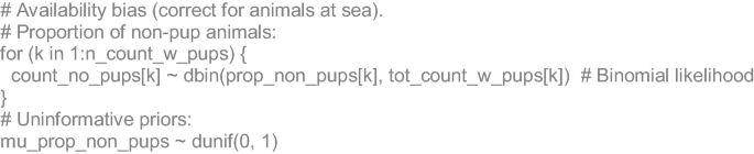
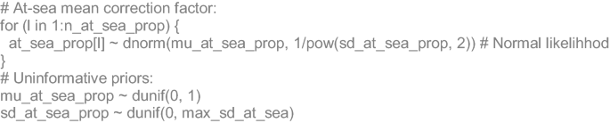
The perception bias of boat-based counts was estimated for all available surveys as the proportion of animals detected from the boat with respect to those detected from the aerial drone photos at each reproductive colony. All proportions were stated as binomial likelihoods, whose inverse main parameters were used as additive correction factors for the annual abundance predictions. We also estimated an availability bias correction factor to add the proportion of animals likely to be at sea when the surveys were made. For that, we used a mean of those proportions reported in a study that compared on-land and at-sea aerial counts at colonies of the same species in the California Current Large Marine Ecosystem⁵⁸. Unfortunately, there was no available information for our study area for this purpose. Since those proportions were with respect to all categories except pups, we had to estimate first the mean proportion of non-pup animals in the Gulf of California from 76 counts with available information (Supplementary Information, Table S1). Then, the correction factor was applied only to non-pup animals for each reproductive colony. Although the proportion of animals foraging at sea can vary as a function of prey availability^43,64, there was no available data or previous information that allowed us to address this dynamically. Therefore, our model assumed this proportion as constant. Since El Partido and El Rasito did not have enough observations during the first 10 years of the time series, and given that both colonies have very limited area available for California sea lions, we set upper truncation limits for their predictions at the beginning of the time series to their maximum total counts available.

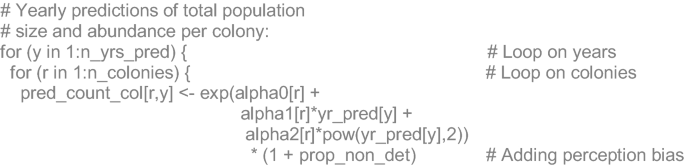
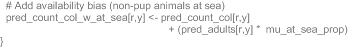
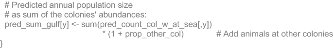
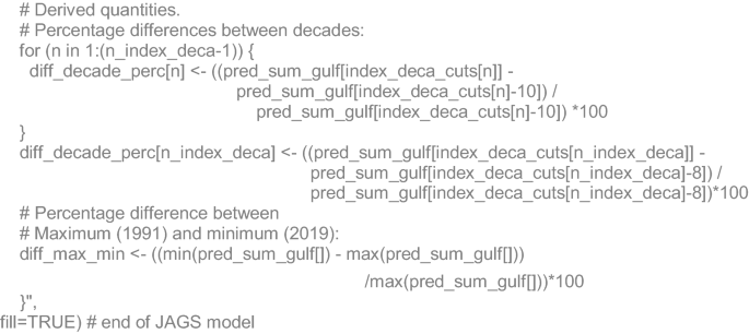
To obtain the annual posterior distributions of the total population size, we summed the annual predictions of abundance at each reproductive colony from 1978 to 2019, all within the same hierarchical Bayesian structure to propagate the uncertainties of the colonies’ estimations⁵³. We also added a final availability bias correction factor to account for the animals likely present at the 16 known non-reproductive colonies during a typical breeding season, based on the counts reported by the only study that included such colonies¹⁸. To better visualize the population size dynamics, we also estimated decadal and maximum percentages of change during the 42-year time series.

100-year anomalies of sea surface temperature

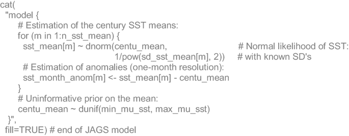
We estimated 25-year running means of sea surface temperature within the Gulf of California and their anomalies from the 100-year mean, from 1920 to 2019 (n = 1,193). This allowed us to filter interannual and decadal signals such as El Niño Southern Oscillation (ENSO) or the Pacific Decadal Oscillation (PDO), respectively, keeping only multi-decadal variability in accordance to the scale of the California sea lion population trend explored in this study. The dataset consisted of predictions from a two-stage reduced-space optimal interpolation procedure, and the superposition of quality-improved gridded sea surface temperature observations onto reconstructions, based on historical ice concentrations at the Earth’s poles⁶⁵. The product was developed by the Met Office Hadley Centre (https://hadobs.metoffice.com/) for use in climate monitoring and modeling, and is freely distributed at a monthly- one-degree resolution by the Environmental Research Division’s Data Access Program of the National Oceanic and Atmospheric Administration (https://coastwatch.pfeg.noaa.gov/erddap/griddap/erdHadISST.html), for which 14 SST prediction points corresponded to the Gulf of California (Fig. 1).

Habitat-based population trend

We fitted a regression model of the 42 annual predictions of California sea lion population size as a function of SSTa at an annual basis, that is, only for the predicted values for July each year, the beginning of the breeding season when the counts were made. For this, we used the means and standard deviations of the posterior distributions of these two parameters, estimated by the two models described above. We tested for incremental polynomial degrees for the regression, but also for pairwise combinations of models through a mixing parameter⁶⁶, which can add flexibility to the curve and increase the explained variability. The best fit was chosen based on the lowest DIC. The results of this function allowed us to calculate geometrically a range of optimum habitat, which was defined as the range of SSTa values at which the population size predictions reached the maximum at the lower and upper 95%-credible interval limits of the curve (Fig. 5). The same approximation was used to calculate the SSTa value at which the population size would reach half of its multi-decadal maximum.

Algebraic and JAGS code details

For the numerical reconstruction of the California sea lion population size in the Gulf of California, all colony counts (C) available (i) were assumed to come from a Poisson likelihood with a logarithmic link, whose parameter (λ) was a function of the year (y) at each reproductive colony (j), which had fixed effects on the relation:

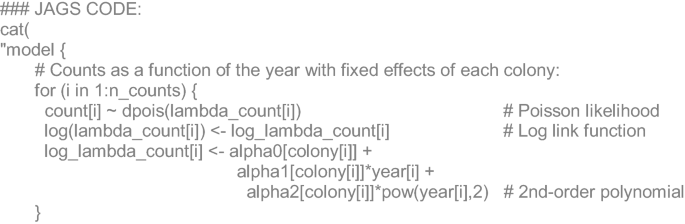
For each reproductive colony (j), boat-based visual counts (V) in 2016 came from a Binomial likelihood, with a mean proportion of detected animals (P_det) respect to the total (T_drone) (i.e. drone-based). The complement proportion of the former corresponds to un-detected animals (P_und):

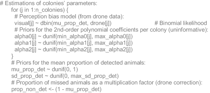
For each survey (k) with available information of pups, non-pup counts (Cnp) were stated to come from a Binomial likelihood with a mean proportion (P_np) respect to the total (T):

For each reference (l) of the proportions published of adult animals at sea (P_ats), a normal likelihood was stated with unknown mean (µ_ats) and standard deviation (σ_ats):

The only total count (TC) available encompassing all reproductive and non-reproductive colonies was stated as the second parameter of a binomial likelihood whose number of animals at the 16 non-reproductive colonies (N_nrc) represents a mean proportion P_nrc:

The annual (y) predictions of animal abundance (A) for the 13 reproductive colonies (r) summed were derived from the function in Eq. 1, adding the proportion of undetected animals (P_und) in visual surveys (i.e. drone-based correction) (Eq. 2):

For each year (y), a number of adult animals (Ad) was estimated at each colony (r), using the mean proportion of non-pup animals (P_np) defined in Eq. 3:

The latter estimate was used to include the correction factor for at-sea animals, not available during the counts, and to obtain the completely corrected annual estimates of abundance (CA) for each colony (r):

The annual population sizes for the 42 years of the series (y) were estimated as the sum of those of the 13 reproductive colonies (i), plus the proportion of animals at non-reproductive colonies (Pnrc):

As secondary derived quantities, we estimated the percentage of decadal (n) changes in the population size and the main percentage decrease from the highest to the lowest:

The analysis of sea surface temperature began by stating the monthly (m) 25-year running means of sea surface temperature (SST) to come from a normal likelihood with the 100-year mean (µ_SST) and known standard deviations (σ_SST; calculated along with the running means). The former was subtracted from the observations to estimate the anomalies (SSTa):

Finally, the ecological model stated that the estimated annual (y) populations sizes (N) followed a Normal likelihood, whose means were a function of the SST anomalies (SSTa) (only for July estimations). The function with the lowest DIC was a mixture between a parabola and a second-order polynomial with θ coefficients, through a mixing parameter (ω). The SSTa estimations were also stated to come from a Normal likelihood with a mean (µ_SSTa) and known standard deviations (σ_SSTa):

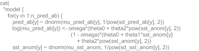
The estimation of the variance explained by this model, the Bayesian R-squared, was based on a vector of errors (i.e. the observed minus the predicted):

Source: Ecology - nature.com