The effect of sediment grain properties and porewater flow on microbial abundance and respiration in permeable sediments

Study site

Sampling was conducted in the subtidal North Sea during RV Heincke cruise 432 in autumn 2014. The sampling site (GPS 54 °10.48′N, 7° 57.44′E) was located in the German Bight between Helgoland and Bremerhaven, where nutrient supply of the rivers Weser and Elbe is fueling enhanced primary production²⁷. The water depth was around 20 meters and typical bottom water velocities range between 7–21 cm s⁻¹ with an additional contribution of the wave orbits by up to 8 cm s^−1 4. The water-temperature during the sampling campaign was 17 °C. Sediments were collected using repeated Van Veen grabs. The upper two centimeters of the sediment were sampled and placed into transport boxes. The procedure was repeated approx. 30 times until sufficient amounts of sediment were sampled. The samples were completely immersed in sea water and additional bottom water was collected and stored in the dark. Organic carbon contents in the water column were on average 0.1 mg POC l⁻¹ (pers. comm. Andreas Neumann, HZG).

Experimental setup

In the lab and approximately 24 hours after retrieval, the sediment was gently homogenized and separated into different grain size fractions using sieves with mesh sizes of 1000 µm, 710 µm, 500 µm and 355 µm in sequential order. This resulted in four grain size fractions that varied in between 355 µm – 500 µm, 500 µm − 710 µm, 710 µm – 1000 µm and <355 µm which approximately reflects the phi scale for sediments (see also Fig. SI 1). The grain size distributions of the fractions were roughly delimited by the mesh size but tailed towards larger grain sizes, which is further discussed below. Four sorted sediment fractions and the original (mixed) sediment were each filled into a flow through reactor (FTR) that was completely submersed in sea water to avoid trapping of air bubbles. The flow through reactors have the advantage that the advective porewater flow can be controlled and microbial processes can be estimated to high accuracy^{3,21,22,25,28}. The FTRs has an inner diameter of d = 10 cm and a length of L_C = 20 cm. This relatively large volume minimizes bias caused by pore water flow along the walls and ensures that enough sediment is present in the FTR to capture the heterogeneity. The length of the flow paths is similar to the typical streamlines length in the upper few centimeter of the permeable sediment^29,30. Radial grooves at the inlet lid and outlet lid of the reactor allowed for a homogenous percolation. Sediment discharge into the tubing was avoided by covering the inlet and outlet lid with a plankton net (80 µm mesh).

The 5 FTRs were positioned vertically, and were continuously supplied with air saturated seawater from 20 L Duran bottles using polyetheretherketone tubing (PEEK) (approx. 3 cm) and TygonTM tubing (approx. 20 cm). The core percolation was driven by peristaltic pumps (ISMATEC, Reglo digital MS-4/6) adjusted to reproduce porewater velocities between 1 cm h⁻¹ to 30 cm h⁻¹ as typically found in permeable sediments (Huettel 1996)²⁵. The cores and reservoirs were kept in the dark at a temperature of 19 °C. Oxygen respiration and NOx (nitrate and nitrite) production rates within the 5 cores were measured at 11 different flow rates over the next 21 days.

Flow characteristics

To assess the homogeneity of the flow within the FTRs and to estimate flow dispersion and sediment porosity, argon saturated seawater was supplied and an argon-breakthrough curve was measured using a membrane-inlet mass spectrometer. The argon-breakthrough represents the cumulative of the porewater age distribution, of which the first moment is the mean retention time r_t and the second moment the longitudinal dispersion D_L = α_Lu, with α_L the longitudinal dispersion coefficient. To allow for a better comparison, the time variable t and longitudinal dispersion D_L were non-dimensionalized using the mean retention time, core length L_c and porewater velocity u: t* = tr_t⁻¹, α_L* = D_Lu⁻¹L_c⁻¹ = α_LL_c⁻¹, where an asterisk denotes non-dimensional variables. For the 1-D scalar-transport equation and boundary conditions as present in the flow-through reactors an analytical solution exists²⁸:

This function is similar to the cumulative function of the Gaussian distribution, where (sigma =sqrt{2{alpha }_{L}^{ast }}) is the standard deviation, C the measured argon concentration at the outlet and C₀ the inlet concentration of argon. Thus, most studies have used Eq. 1 as a fit function for the breakthrough curves³¹. Here, we directly estimate the unknown sediment porosity via the retention time and the flow dispersion from the second moment of the porewater age distribution²⁸.

When measuring reaction rates in FTRs the reactants should not be depleted before the porewater reaches the outlet. We employ the Damköhler number to express the specific rates of reaction and transport (see also appendix SI5):

where L is the length scale, θ the porosity, R the volumetric oxygen consumption and C_in the reservoir oxygen concentration. In case Da >1 the solute would be depleted within the core. To account for flow dispersion the longitudinal dispersion coefficient is added to the core length (L={L}_{c}+sqrt{2{alpha }_{L}u{r}_{t}}) causing L to be 10% to 40% larger than the core length (L_c) itself. This is the length scale to which dispersion would affect the respiration rate measurements.

Sediment characterization

Grain size distributions from the size fractionated sediments were measured using a laser diffraction particle size analyzer (Beckman Coulter, LS 200) and binned into 92 size classes ranging from d₀ = 0.4 µm to d₁ = 2000 µm. Prior to measurements the samples were acidified to remove carbonates. From the measured grain size distribution the theoretical surface area to volume ratio S_V,T can be calculated:

where θ is the porosity, p(d_g) is the probability density function of the respective sediment fractions and d_g the diameter of the grains. Equation 3 assumes spherical grains, which is not necessarily the case. Therefore, the surface area per mass (Am⁻¹) was also measured via nitrogen adsorption using a Brunauer-Emmett-Teller analyzer (Quantachrome Quantasorb Jr.) (see also Mayer¹²). Based on density ρ_p of the particles the surface-to-volume ratio can be calculated:

The permeability of the sediment fractions was estimated by measuring the pressure drop along the flow through reactor. Along the flow direction two tubes were attached to the FTR in δ = 10 cm distance. The pressure drop is visible as a difference between the water heads (h₁-h₀) in the tubes. Based on Darcy’s law the porewater velocity can be calculated:

where k is the permeability, μ the dynamic viscosity and ∇p the pressure gradient. The pressure gradient can be determined by the hydrostatic pressure drop between the tubes: (nabla p=rho g({h}_{1}-{h}_{0}){delta }^{-1}), where ρ is the water density, g the acceleration by gravity. Substitution and rearranging yields:

The sphericity of sand grain is defined as the ratio of the surface area of a sphere to the surface area of the sand grain at the same volume³². However, accurate determination would require 3D-reconstructions of individual sand grains which would severely limit the feasible sample size. To allow for larger throughput of sand grains, we estimated the sphericity in a 2D plane by determining the perimeter of the sand grains relative to the perimeter of a circle at the same area. Sand grains were subsampled from the flow through reactors and transferred onto petri dishes for determination of 2D-sphericity. Photographic images were taken at 25x magnification using a SLR camera (Nikon D90) attached to an inverse microscope (Leica DMI 6000 B).

The images were processed using the image processing toolbox of Matlab (Mathworks 2018 b). Briefly, the image was inverted and binarized using a threshold of 0.8. In the resulting images, sand grains appeared as connected white areas, which were identified using an automated script, and subsequently the edges of the connected white areas were traced (see Fig. SI 4b). These edges represent the perimeter p of the sand grains. The area A was determined by integrating the connected white pixels. Based on A and p the sphericity indicator S_P can be determined ({{boldsymbol{S}}}_{{boldsymbol{P}}}=frac{sqrt{2{boldsymbol{pi }}{boldsymbol{A}}}}{{boldsymbol{p}}}). In total 45 images were taken and 5–15 sand grains were processed per image. In total, approximately 400 sand grains were individually analyzed.

For carbon content analysis, sediment samples were taken from the FTRs and frozen at −20 °C. The sediment samples were dried, ground, acidified, and subsequently the total organic carbon content was determined using an elemental analyzer (Elementar, vario TOC cube).

Cell counts

After ten days of incubation, the FTRs were opened for a short time period and 5 cm of sediments were removed, then 5 ml sediment samples were taken to quantify the total cell abundance. The FTRs were subsequently closed again, taking care that no preferential pathways had been created. Approximately 0.5–1 ml of sediment were fixed in a formaldehyde solution (1% in phosphate buffered saline, PBS) at room temperature followed by repeated centrifugation and replacement of the supernatant with the PBS solution. Cells were then extracted from the grains by sonication (Sonopuls HD70) with a UW 70 sonication probe (Bandelin) following the protocols of Probandt et al.³³ and Kuwae, T. and Hosokawa, Y.³⁴. Each sample was sonicated 5 times for 30 seconds at a low intensity (25% power, cycle 20). Supernatant was collected and replaced by the PBS solution between the sonication steps. Subsequently, 200 µl to 500 µl of supernatant was subsampled and diluted in 10 mL PBS:EtOH solution. Cells were then filtered on 0.2 µm Isopore membrane filters (Millipore). Finally, filters were dried at 40 °C and embedded in 0.1% agarose gel (Biozym, low melting temperature gel with strength larger than 800 g cm⁻²) and stored at −20 °C.

Cells were enumerated after staining with SYBR Green I (invitrogen). The 10000x SYBR Green I stock solution was diluted 1:50 in sterile 1 mol l⁻¹ Tris HCl with a pH of 7.5. Subsequently, 60 µl were transferred onto a petri dish. Filter pieces were stained for 20 minutes and stabilized in mounting medium (Mowiol 4–99 Sigma). Cells were counted using an epifluorescence microscope (Leica DMI6000B) at an excitation wavelength of 498 nm. For each filter 28 to 61 randomly chosen grids were counted, encompassing an area of 1000 µm² with at least 1300 SYBR Green signals in two biological and three technical replicates.

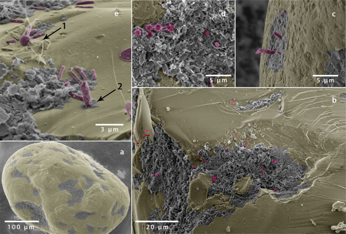
In situ colonization on sand grains

Scanning electron microscopy was used to visualize the microbial community on surfaces of sediment grains. Sediment was fixed in 2.5% glutaraldehyde in 0.1 M sodium cacodylate buffer at pH 7.2 and post fixed in OsO4 in the same buffer. Sediment was then washed in ethanol-water mixtures with increasing concentration (30%, 50%, 70%, 90% and 100%) for 15 minutes at each step, and then dried in a critical point dryer (Leica EM CPD 300). The sand grains were then sprinkled onto double sided conductive carbon adhesive tabs. Imaging was performed using a Quanta 250 FEG scanning electron microscope (FEI) with an acceleration voltage of 2 kV. The grey scale scanning electron micrographs were colorized using Photoshop (Adobe, CS 9) to identify bacteria and detritus.

Oxygen respiration, denitrification and combined nitrate- nitrite production

Oxygen respiration, denitrification and combined nitrate- nitrite production were estimated by measuring the difference of the respective solutes between inlet (C_in) and outlet (C_out) of the flow through reactor:

where ({r}_{t}={L}_{c}{u}^{-1}) is the mean retention time, with L_c the length of the core, u the porewater velocity, calculated from the pump volume f ((u=f{A}^{-1}{theta }^{-1})), and θ the porosity.

Oxygen was continuously measured using optode flow-through cells (OXFTC, Pyroscience coupled to a 4-channel Firesting amplifier, Pyroscience). For each of 11 different flow rates, oxygen consumption was measured simultaneously on the five different sediment fractions. Flow rates were typically changed after 24 hours. After adjusting the pump volume stable consumption rates indicated that a steady state had been reached. This occurred typically after 1.5 times the mean retention time, i.e., the time a water parcel travels from inlet to outlet. Various flow rates were applied in a random order to ensure that changes in oxygen consumption rates were related to change in flow rates, rather than to temporal changes of the microbial community or organic carbon content. Furthermore, in a number of cases, rate determinations were repeated based on randomly chosen flow rates.

Nitrification, anammox, DNRA and denitrification have all been shown to occur in sandy sediments, however in the subtidal sands of the North Sea, nitrification and denitrification are the dominant processes⁵. Therefore, we focus on nitrification under oxic conditions and denitrification rates under anoxic conditions. During oxic incubations, inlet and outlet porewater was subsampled for NOx concentrations and frozen at −20 °C. Nitrite and nitrate concentrations were measured on a CLD 60 Chemiluminescence NO analyzer (Ecophysics)³⁵ and rates were calculated according to Eq. 7.

After 3 weeks of oxic incubation, the seawater reservoir water was degassed by purging with argon and amended with 70 µmol l^{−1 15}NO₃⁻ and subsequently Ar, ²⁸N2, ²⁹N2 and ³⁰N2 was continuously measured at the outlet via a membrane-inlet mass spectrometer (GAM200, IPI). Denitrification rates were calculated based on the equations described in³⁶. For the denitrification experiments only one flow rate was used resulting in porewater velocities between 9 cm h⁻¹ to 12 cm h⁻¹ depending on the porosity of the respective sediment fractions. These porewater velocities represent an intermediate range of measured porewater velocities in nature²⁵.

Source: Ecology - nature.com