The impact of antimalarial resistance on the genetic structure of Plasmodium falciparum in the DRC

Study populations

Chelex-extracted DNA samples from dried blood spots, collected as part of the 2013–2014 DRC Demographic Health Survey (DHS), were tested using quantitative real-time PCR to detect Plasmodium falciparum lactate dehydrogenase (pfldh)^32,33. Previously published DRC samples¹⁰ were included (n = 589), and used to set a Ct threshold of <30 for inclusion for sequencing, which was applied to the remaining DRC samples (n = 1450), resulting in a total of 2039 DRC samples sent for sequencing. These samples represented 369 of the overall 539 DHS clusters. In addition, dried blood spot samples from four further counties were used: Ghana (n = 194), Tanzania (n = 120), Uganda (n = 63), and Zambia (n = 121). Samples from Ghana were collected in 2014 from symptomatic RDT and/or microscopy positive individuals presenting at health care facilities in Begoro (n = 94) and Cape Coast (n = 98)³⁴. Samples from Tanzania were collected in 2015 from symptomatic RDT-positive patients of all ages at Kharumwa Health Center in Northwest Tanzania³⁵. Samples from Uganda were collected in 2013 from RDT-positive symptomatic patients at Kanungu in Southwest Uganda³⁶. Finally, samples from Zambia were collected in 2013 from RDT-positive individuals from a community survey of all ages in Nchelenge District in northeast Zambia on the border with the DRC. All non-DRC samples were Chelex extracted, except for the Ghanaian samples which were extracted using QiaQuick per protocol (Qiagen, Hilden, Germany). This study was approved by the Internal Review Board at UNC and the Ethics Committee of the Kinshasa School of Public Health.

Design of MIP panels

We used two distinct MIP panels—a genome-wide panel designed to capture overall levels of differentiation and relatedness, and a drug resistance panel designed to target polymorphic sites known to be associated with antimalarial resistance (Supplementary Note 1). When selecting targets for the genome-wide panel, we used the publicly available P. falciparum whole-genome sequences provided by the Pf3k and P. falciparum Community projects from the MalariaGEN Consortium. This consisted of sample sets from Cameroon (n = 134), DRC (n = 285), Kenya (n = 52), Malawi (n = 369), Nigeria (n = 5), Tanzania (n = 66) and Uganda (n = 12) (Supplementary Data 1). The genomic sequence from these samples underwent alignment, variant calling, and variant-filtering following the Pf3k strategy consistent with the Genome Analysis Toolkit (GATK, version 3.6 unless otherwise indicated) Best Practices with minor modifications^37,38,39,40. Full details of the bioinformatic pipeline used in MIP design are given in the Supplementary Note 1. Samples from Nigeria and Uganda were dropped after variant calling due to small sample sizes, and the final filtered sequences were used to calculate Weir and Cochran’s F_ST⁴¹ with respect to country for each biallelic locus. The 1000 loci with the highest F_ST values were considered for MIP design as phylogeographically informative loci. Of these 1000 potential loci, 739 were identified as regions that were suitable for MIP-probe design. Separately, from the combined SNP file, we identified 1595 loci that had a minor-allele frequency >5%, had an F_ST value between 0.005 and 0.2, and were annotated by SnpEff (version 4-3t) as functionally silent mutations. These loci were identified as putatively neutral SNPs, and 1151 were found to be suitable for MIP design. The distribution of MIPs is shown in Supplementary Fig. 14 and MIP sequences and targets are shown in Supplementary Data 3.

MIP capture and sequencing

In addition to patient samples, control samples were known mixtures of 4 strains of genomic DNA from malaria at the following ratios: 67% 3D7 (MRA-102, BEI Resources, Manasas, VA), 14% HB3 (MRA-155), 13% 7G8 (MRA-154) and 6% DD2 (MRA-156). They were also represented at two different parasite densities (29 and 467 parasites/µl). MIP capture and sequencing library preparation were carried out as described in the Supplementary Note 1¹⁰. Drug resistance libraries were sequenced on Illumina MiSeq instrument using 250 bp paired end sequencing with dual indexing using MiSeq Reagent Kit v2. Genome-wide libraries were sequenced on Illumina Nextseq 500 instrument using 150 bp paired end sequencing with dual indexing using Nextseq 500/550 Mid-output Kit v2.

MIP variant calling and filtering

MIP variant calling is summarized in the Supplementary Note 1¹⁰. Within each sample, variants were dropped if they had a Phred-scaled quality score of <20. Across samples, variant sites were dropped if they were observed only in one sample, or if they had a total UMI count of <5 across all samples. This data set was considered the final raw data used for additional filtering.

Additional filters were applied to both genome-wide and drug resistance datasets prior to carrying out analysis. Sites were restricted to SNPs, and in the case of the genome-wide panel these were filtered to the pre-designed biallelic target SNP sites. Any variant that was represented by a single UMI in a sample, or that had a within-sample allele frequency (WSAF), UMI count of allele/total UM less than 1%, was eliminated. Any site that was invariant across the entire dataset after this procedure was dropped. Samples were assessed for quality in terms of the proportion of low-coverage sites, where low-coverage was defined as fewer than 10 supporting UMIs. Samples with >50% low-coverage loci were dropped. Variant sites were then assessed by the same means in terms of the proportion of low-coverage samples, and sites with >50% low-coverage samples were dropped. Samples were then combined with metadata, including geographic information, and were only retained if there were at least 10 samples in a given country. This resulted in dropping Tanzanian samples from the drug resistance dataset, but no other countries were dropped. Post-filtering, genome-wide data consisted of 1382 samples (DRC = 1111, Ghana = 114, Tanzania = 30, Uganda = 45, Zambia = 82) and 1079 loci, and drug resistance data consisted of 674 samples (DRC = 557, Ghana = 29, Uganda = 43, Zambia = 45) and 1000 loci. The complete bioinformatic pipeline is shown in Supplementary Fig. 15.

Complexity of infection

We applied THE REAL McCOIL (v2) categorical method to the SNP genotyped samples to estimate the COI of each individual¹³. Details of the analysis are in the Supplementary Note 1.

Analysis of population structure

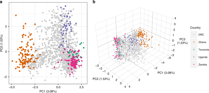
WSAFs were calculated for all genome-wide SNPs, with missing values imputed as the mean per locus. Principal component analysis (PCA) was carried out on WSAFs using the prcomp function in R version 3.5.1. The relative contribution of each locus was calculated from the loading values as (left| {l_i} right|/mathop {sum}nolimits_{i = 1}^L {left| {l_i} right|}), where (left| {l_i} right|) is the absolute value of the loading at locus (i), and (L) is the total number of loci. PCA results were explored in a spatial context by taking the mean of the raw principal component values over all samples in a given DHS cluster, and plotting this against the geoposition of the cluster.

Identity by descent analysis

Pairwise IBD was calculated between all samples from the genome-wide SNPs. We used Malécot’s⁴² definition of (f) as the probability of identity by descent, where (f_{{mathrm{uv}}}) can be defined as the probability of a randomly chosen locus being IBD between samples ({mathrm{u}}) and ({mathrm{v}}). At locus ({mathrm{i}}), let (A) denote the reference allele, which occurs at population allele frequency (p_{mathrm{i}}), and let (a) denote the non-reference allele, which occurs at population allele frequency (q_i = 1 – p_{mathrm{i}}). Assuming that both samples ({mathrm{u}}) and ({mathrm{v}}) are monoclonal, let (X_{{mathrm{ui}}}) denote the observed allele at locus ({mathrm{i}}) in sample ({mathrm{u}}), and equivalently let (X_{{mathrm{vi}}}) denote the observed allele in sample ({mathrm{v}}). Then the probabilities of all possible observed allele combinations between the two samples can be written:

from which we can calculate the likelihood of a given value of (f_{{mathrm{uv}}}) over all loci as:

In practice, population allele frequencies ((p_{mathrm{i}})) were calculated using the mean WSAF for that locus over all samples. Samples were then coerced to monoclonal by calling the dominant allele at every locus. The likelihood was evaluated using Eq. (2) in log-space for a range of values of (f_{{mathrm{uv}}}) distributed between 0 and 1 in equal increments of 0.02. The maximum likelihood estimate (hat f_{{mathrm{uv}}} = {rm{argmax}}_{mathrm{f}},L(f|X_{mathrm{u}},X_{mathrm{v}})) was calculated between all sample pairs. Hereafter the terms IBD and (hat f_{{mathrm{uv}}}) are used interchangeably.

The validity of this method of coercing samples to monoclonal before estimating IBD via maximum likelihood was rigorously explored in a simulation-based analysis. First, a simulation framework was created that permitted simulating samples with variable polyclonality. This framework is described in detail in Supplementary Note 2. Second, true vs. estimated IBD were plotted for a range of polyclonal settings and a range of sub-sampled data sizes going down from the true data to 500, 100, and 20 SNPs. Any positive or negative bias introduced by forcing samples to be monoclonal would be reflected and quantified in this plot.

Mean IBD was calculated within and between DHS clusters, and compared using a two-sample t-test. Sample pairs were also binned into groups based on geographic separation (great circle distance) in 100 km bins, with an additional bin at distance 0 km to capture within-cluster comparisons. Mean and 95% confidence intervals of IBD were calculated for each group. Finally, sample pairs with IBD > 0.9 were identified, and explored in terms of their WSAFs and their spatial distribution.

Estimating mutation prevalence from drug resistance panel

Given previous findings of an East–West divide in molecular markers of antimalarial resistance in the DRC^8,9, all samples in the DRC were divided by geographically weighted K-means clustering into two populations. The prevalence of every mutation identified by the drug resistance MIP panel was then calculated in East and West DRC, as well as at the country level. Prevalences in each DHS cluster were used to produce smooth prevalence maps using PrevMap version 1.4.2 in R⁴³.

Analysis of monoclonal haplotypes

Results of the previous COI analysis on the genome-wide SNPs with THE REAL McCOIL were used to identify samples that were monoclonal with a high degree of confidence. Samples were defined as monoclonal if the upper 95% credible interval did not include any COI greater than one. This resulted in 408 monoclonal samples, of which 143 overlapped with the drug resistance MIP dataset and therefore could be used to explore the joint distribution of mutations in drug resistance genes. 107 of these were from DRC. Analysis focussed on the dhps and crt genes. Raw combinations of mutations were visualized using the UpSet package in R²¹, and the spatial distribution of haplotypes was explored by plotting these same mutant combinations against DHS cluster geoposition.

Extended haplotype homozygosity analysis

In order to improve our power to detect hard-sweeps and capture patterns of linkage-disequilibrium with EHH statistics among putative drug resistance SNPs, we combined the genome-wide and the drug resistance filtered biallelic SNPs into a single dataset (Supplementary Note 1). All associated EHH calculations were carried out using the R-package rehh (version 2.0.4), and were truncated when fewer than two haplotypes were present or the EHH statistic fell below 0.05^44,45. In addition, we allowed EHH integration calculations to be made without respect to “borders,” which were frequent due to the MIP-probe design. Although this would result in an inflated integration statistic if the EHH statistic had not yet reached 0 within the region of investigation, this problem was mitigated by only comparing between subpopulations, and not between loci. EHH decay, bifurcation plots, and haplotype plots were adapted from the rehh package objects and modified using ggplot⁴⁶.

Reporting summary

Further information on research design is available in the Nature Research Reporting Summary linked to this article.

Source: Ecology - nature.com