Waterfowl occurrence and residence time as indicators of H5 and H7 avian influenza in North American Poultry

Animal protocols statement

The authors confirm that all methods were carried out in accordance with relevant guidelines and regulations and that all experimental protocols were approved by the appropriate institutions and licensing committees. Protocols for capturing, handling, and instrumenting blue-winged teal included in this study were reviewed by institutional animal care and use committees (USGS Alaska Science Center Animal Care and Use Committee Animal Use permit no. 2014–5 and the University Committee on Animal Care and Supply University of Saskatchewan Animal Use protocol no. 20070039) and carried out under federal authority (US Department of the Interior Federal Bird Banding permit nos. 09072 and 23792, Federal Fish and Wildlife permit no. MB779238-2, Environment Canada Migratory Bird Banding permit no. 10458R).

Study domain and bird telemetry

Our study area encompassed North America between 14.5° and 60.0° North Latitude and −137.5° and −66.2° West Longitude. This area includes the conterminous United States, Mexico, Cuba, the Bahamas, and major portions of Canada. Forty-two adult, male blue-winged teal were captured and marked. Twelve birds were captured on their summer range in the Saskatchewan and Alberta Canadian Provinces during August 11–15, 2013, with the remaining thirty birds captured at wintering areas along the Texas and Louisiana Gulf Coast in the United States during March 17–22, 2015. All birds were marked with 9.5 gram, solar-powered Platform Transmitter Terminals (PTTs) manufactured by Microwave Telemetry, Inc., Columbia, Maryland (USA) and then released in close proximity to their respective capture locations. The PTTs were attached using a Teflon harness secured over the sternum to have a dorsally extended antenna as outlined by Takekawa et al.⁴⁶. The PTTs were programmed to have a regular duty cycle with a 10 hour on period every 48 hours. We used the Argos Data Collection and Location System (CLS America, Incorporated, Largo, Maryland, USA) to receive transmissions, which provided Doppler-based location estimates, a movement activity indicator, and a class index reporting the quality of each location estimate. To prepare telemetry for statistical modeling, we first applied a filtering algorithm⁴⁷ and then manually inspected movements and activity sensor records to exclude dates following likely bird mortality or PTT detachment. Locations exhibiting an unchanged activity indicator over two or more duty cycles were removed from the telemetry dataset. Table 1 details the bird-specific number of locations retained for analysis following data cleaning. Animations depicting the wild bird’s used in this study and downloadable telemetry data are available from the U.S. Geological Survey, Alaska Science Center, Wildlife Tracking Data Collection (https://doi.org/10.5066/P9Z9BA9F)⁴⁸.

Environmental data

To characterize habitat and environmental conditions over the study area, we utilized 250 meter resolution gridded soils data⁴⁹, the Global Topographic 30 Arc-Second Digital Elevation Model available from the U.S. Geological Survey (USGS) Earth Resources Observation and Science Center (https://www.usgs.gov/centers/eros), the 300 meter 2009 GlobCover Land Cover Maps provided by the European Space Agency (http://due.esrin.esa.int/page_globcover.php), and 30 meter resolution topographic roughness and topographic wetness indices provided by the ENVIREM dataset⁵⁰. Because our goal with incorporating environmental variables was to characterize waterfowl habitat broadly and not to infer species-specific preferences or tolerances, we decomposed gridded soils data (17 different soil attributes) and elevation derived variables (topographical roughness, topographical wetness, elevation, and slope) using separate Principal Components Analyses and selected the resulting first component from each to represent soil and topographical conditions respectively. The correlation of the retained first component to other attributes included during decomposition are provided for soils in Table 2 and topography in Table 3. In addition to simplifying our analysis, the decomposition of variables also aided in avoiding multicollinearity issues during the model fitting process⁵¹. Recognizing the critical importance of wetlands and surface waters to waterfowl, we also calculated the Euclidean distance (km) of each telemetry location to the nearest surface water class in the GlobCover land cover dataset using the Program R⁵² and the spatstat package⁵³. As detailed in subsection 2.6, we modeled distance to water as a non-linear covariate to avoid treating water presence as a bird occurrence prerequisite.

Poultry and human density data

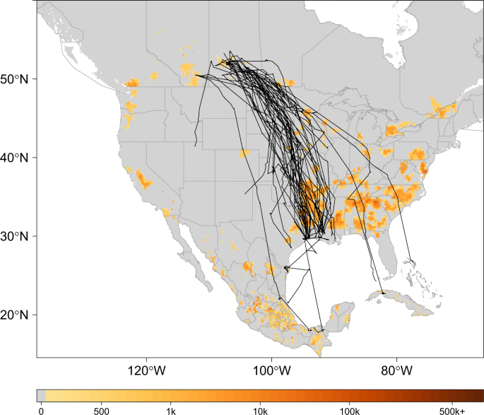
For estimates of poultry abundance, we used the chicken and duck raster layers from the Food and Agriculture Organization of the United Nations (FAO) Gridded Livestock database⁵⁴. The rasters were provided at a 0.083333 decimal degree resolution and report the number of poultry head per square kilometer (head/km²). Human population density estimates were obtained as a continuous raster (30 meter) from NASA’s Socioeconomic Data Center that gave the number of persons per square kilometer (persons/km²)⁵⁵. The distribution of poultry abundance relative to our study domain is shown in Fig. 1 with telemetry tracks overlaid for marked birds.

Figure 1

Track Map. Telemetry tracks for 42 blue-winged teal over grid depicting poultry abundance⁵⁴. Black lines show individual bird tracks, legend describes estimated number of poultry (chickens and ducks) per km². To better display poultry abundance in this figure, zero was defined as less than 100 poultry/km².

Full size image

Avian influenza event in poultry data

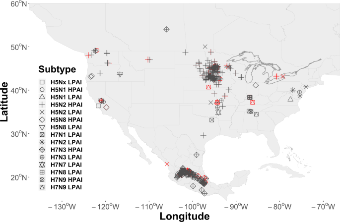
AIP data were obtained from the web-based Global Animal Disease Information System (EMPRES-i) maintained by the FAO (http://empres-i.fao.org/eipws3g/, accessed 12/01/19). EMPRES-i is intended to support veterinary services and related organizations by providing access and analysis of global animal disease information. We initially downloaded all AIP data for the period between January 01, 2004 and December 01, 2019 and then filtered records to include only those with an FAO “Confirmed” status, geographically located within our study domain, affecting commercial poultry, and associated with virus subtypes having a H5 or H7 hemagglutinin surface protein. The H5 and H7 subtypes were chosen due to our interest in the HPAI pathotype, however, both HPAI (n = 440) and LPAI (n = 49) events were included in the resulting 489 record dataset. A secondary consideration in limiting the study to the H5 and H7 subtypes was that these subtypes are required to be reported to the World Organization for Animal Health (OIE) giving us some confidence in our sample. This is not the case with other virus subtypes, which are reported voluntarily and may therefore introduce sample bias. As a final step in preparing AIP data, we randomly selected 97 AIPs (approximately 20%) as a hold-out dataset to aid in later model validation. Locations of all events are shown by virus subtype in Fig. 2.

Figure 2

Locations of Avian Influenza Events (AIP) by virus subtype. AIP cover the period 2004–2019 and included 440 events used for model training and 49 (20%) randomly selected for model validation. Locations shown in the color red signify those retained for validation.

Full size image

Statistical analysis

We constructed a two-level, spatially explicit model with shared components to evaluate the spatial and temporal relationship of waterfowl to AIPs across North America. The model’s first level estimated waterfowl residence time across the study area, whereas, the model’s second level provided the probability of an AIP as conditioned on that waterfowl residence time. More generally, our model can be represented as:

where the first level [Eq. 1] estimates waterfowl residence time (y₁) at locations i ((i=1,2,3,ldots ,n)) and the second level [Eq. 2] gives AIP probability (y₂) based on the past event (H5 or H7 AI detection) occurrence or absence (1, 0) at location i and conditioned on waterfowl residence time (({y}_{1})). This formulation offers independent intercepts for each model level (({alpha }_{j})), covariate matrices ((beta cdot {X}_{j})) for level-specific linear and fixed effects, and uncorrelated error terms (({e}_{j})). Although independent spatial fields (({Z}_{1}) and ({Z}_{2})) help account for spatial dependencies within each model level, we added a third spatial field (({Z}_{shared})) to explicitly serve as a shared scaling parameter between model levels^56,57. The shared field is a re-scaled copy of ({Z}_{1}) that controls for spatial autocorrelation and interaction occurring between waterfowl telemetry and AIP locations. As an initial step in specifying the spatial fields, we created a triangulated mesh over our study area using procedures described by Lindgren and Rue⁵⁸. In addition to facilitating parameterization of the continuous spatial fields needed to account for spatial dependencies, the mesh provided a computationally efficient alternative to characterizing our continent-sized study domain using raster grids or areal polygons. The mesh included 9,555 nodes and had an outer extension large enough to avoid edge effects around study area boundaries. Due to our large study area, the mesh was projected using three-dimensional Cartesian coordinates scaled to one Earth radius (6,371 km). As a component of sensitivity analyses, meshes constructed with 4,897 nodes and 12,651 nodes were also evaluated and found to exhibit a mean spatial effect within 10% of that estimated using 9,555 nodes; therefore, we selected the middle-ground to balance precision and processing time.

To accommodate the joint modeling approach, our dependent variable was structured as a bivariate matrix with the first column corresponding to residence times calculated from telemetry data and the second column being a vector of 1’s and 0’s designating a past AIP occurrence (1) or absence (0) at each location. Because bird and AIP locations did not always geographically coincide, our model incorporated spatial misalignments; however, this was not problematic as the model is capable of providing estimates across continuous space and for all locations within the study domain⁵⁶. To acquire initial residence time estimates for model fitting, we disaggregated individual bird telemetry tracks (Fig. 1) into 1 minute temporal intervals and then summed them based on mesh node proximity (i.e., “natural neighborhoods”). To achieve this, we performed a Voronoi tessellation around mesh nodes to identify each node’s respective area of influence⁵⁶. Area of influence refers to the bounded area surrounding each node in which all enclosed locations share that node as their closest point⁵⁹. The process used to disaggregate tracks into equal time intervals was adapted from Sumner⁶⁰, but, modified to allow for summation of time intervals based on our tessellated neighborhoods as opposed to a regular grid. Each column of the bivariate matrix exhibited a different distribution, therefore, we specified model likelihoods as,

where, residence time was always a positive value with shape and scale parameters (({a}_{i},{b}_{i})) such that ({a}_{i}/{b}_{i}={mu }_{i}=E({v}_{i})cdot Exposure). Defining Exposure as the area of each node’s tessellated neighborhood, the residence-time linear predictor ({v}_{i}) was of the form,

here, a log link function was used with ({alpha }_{1}) as the intercept, ({beta }_{1}) the soil variable coefficient, ({beta }_{2}) the topography coefficient, ({beta }_{3}) the coefficient for linear distance to nearest wetland, and ({Z}_{1}) as the spatial field to control for spatial dependencies and other unobserved latencies (errors) that may have resulted from the aggregating process undertaken to estimate residence time.

The corresponding linear predictor for the binomially distributed AIP occurrence vector relied on the logit function and was specified as,

where ({alpha }_{2}) is an intercept, ({beta }_{1}) is the coefficient for poultry density and ({beta }_{2}) is the human population density coefficient. As described for Eq. 2, ({Z}_{2}) provides a spatial field to account for domain-wide spatial dependencies and latencies among AIP locations, whereas, ({Z}_{shared}) controls for the spatial relationship between AIP and waterfowl locations. To supplement poultry and human population density variables, we developed two additional model covariates; one to account for fine-scale spatial structure among AIP locations (({f}_{1},{rm{Cluster}})) and the second to examine the temporal relationship between seasonal waterfowl migration and the timing of AIPs (({f}_{2},{rm{Displacement}})).

As shown by Fig. 2, the geographic distribution of AIPs across North America exhibits broad regional coverage (e.g., the Midwestern U.S.) as well as more localized or concentrated “clustering“ at some locations (e.g., Jalisco, Mexico or Minnesota, USA). We speculate that the epidemiological processes that gave rise to the fine-scaled, cluster patterns were likely different than those that instigated the broad-scale, region-wide coverage. More specifically, it is possible that farm-to-farm transmission or “lateral spread” produced the observed clusters, whereas, the broader coverage may be better explained by waterfowl introduction (see, Discussion for further explanation). We chose to address these different multi-scaled spatial processes using two separate spatial covariates. The spatial field (({Z}_{2})) was used as a domain-wide spatial covariate, while fine-scale spatial structure associated with AIP clusters was modeled using a random walk process across AIP nearest neighbor distances (km). As used here, a random walk (({f}_{1},{rm{Cluster}})) is similar to a regression spline in that it permits distances between AIPs to follow a smooth, curvilinear distribution without assuming a mean response. The benefit of using the fine-scale spatial effect is that it quantifies the spatial variability due to proximity between AIP locations, thereby, reducing the model’s capacity to attribute that variation to waterfowl or other covariates.

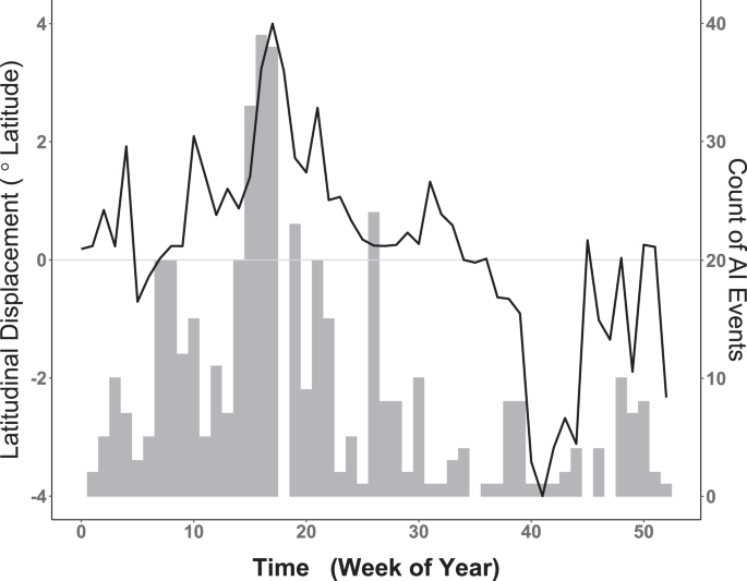
As with clustering, a random walk was also implemented to quantify the temporal relationship between seasonal waterfowl migration and the timing of AIPs. As shown in Fig. 3, summing raw AIP counts (all years, 2004–2019) by week reveals an apparent correlative relationship of AIP timing to the mean weekly latitudinal displacement exhibited by waterfowl. To capture the timing of waterfowl movement as a model covariate, we calculated latitudinal displacement by finding the weekly mean latitude occupied by marked birds (all years, 2013–2016) and then performing a one-week lag subtraction between weeks. The function ({f}_{2},{rm{Displacement}}) introduces the resulting time-ordered vector as a non-parametric, dynamic effect that captures waterfowl latitudinal change at each weekly time step t ((t=1,2,3,ldots ,52)).

Figure 3

Weekly comparison of historic AI Events (AIPs) with waterfowl latitudinal displacement. Left vertical axis corresponds to smooth black line and represents weekly latitudinal displacement of waterfowl measured in degrees latitude. Horizontal axis provides the week of year. Dotted line intersecting zero signifies no net waterfowl displacement, with portions above zero indicating relative northward movement and portions below showing net southward change. Vertical axis at right corresponds to gray histogram for the weekly counts of all AIP summed over the period 2004–2019. Note apparent temporal correlation between waterfowl spring migration (Weeks 5–18) and increasing AIP as well as that between fall migration (weeks 35–42) and decreased AIP counts.

Full size image

We used a Penalized Complexity (PC) framework^61,62 for the three spatial fields (({Z}_{j})) with priors scaled to one Earth radius to reflect the size and projection of our 3D triangulated mesh. Because all spatial fields occurred over a common mesh and spatial domain, PC priors were set with both the spatial range and standard deviation quantile and probability: ({rho }_{0}=1) and ({p}_{rho }=0.5). The PC priors for the spatial effect were intended as non-informative and can be interpreted as specifying a 0.5 probability that the spatial range is within 6,371 km (i.e., one Earth radius). Sensitivity analyses for probability values between 0.2 and 0.8 in 0.1 increments assuming a ({rho }_{0}=1) revealed minimal change to model estimates. Flat PC priors were likewise applied for the random walk effects modeled as ({f}_{1},{rm{Cluster}}) and ({f}_{2},{rm{Displacement}}), which were specified as (mu =1) and (alpha =0.0001). We then combined priors and likelihoods using Integrated Laplace Approximation⁶³.

In addition to performing joint estimation of waterfowl residence time and AIP occurrence probability as described above, we also explored an alternative model formulation to jointly estimate waterfowl occurrence probability with AIP occurrence probability. That is, rather than using residence time to inform AIP probability, the alternate formulation used mere waterfowl occurrence to estimate AIP probability as a way of comparing the relative importance of bird presence versus the amount of time spent at a location. Under the alternative model, we assumed that all locations with a residence time equal to, or exceeding 24 hours constituted an occurrence (1) with unobserved locations (0) used to characterize background environmental conditions. To correspond with the derived presence-background vector, we substituted a binomial likelihood for the gamma in Eq. 3, and exchanged a logit link function for the log. The alternative binomial-binomial configuration included all of the same spatial and environmental covariates as described for the Gamma-binomial.

Model evaluation

To evaluate model accuracy, we performed model-based estimation for each AIP location and event time in the independent testing dataset that was randomly selected and excluded from model development. We calculated the percent correctly classified (PCC), sensitivity (proportion of correctly predicted presences), specificity (proportion of correctly predicted absences), and the area under the receiver operating characteristic curve (AUC) using the Presence Absence R package⁶⁴, and then estimated the True Skill Statistic (TSS) by subtracting a value of one from the sum of the sensitivity and specificity estimates⁶⁵. We also used tools available in the Presence Absence package to determine the probability thresholds that best maximize sensitivity, specificity, and the TSS. Probability thresholds were determined by comparing the input data to model estimates to ascertain the probability value (threshold) that best captured known disease occurrences.

In addition to validating with an independent out-of-sample testing data set, we applied a comparative approach to assess the overall performance of our joint waterfowl residence time and AIP occurrence probability model. In total, seven different models were constructed and then compared to the full joint model detailed in subsection 2.6, one of which (Model6) was the alternative formulation described in the closing paragraph of subsection 2.6. Recognizing that application of parsimony metrics to spatial models can be problematic^66,67, we chose three different parsimony measures; the deviance information criterion (DIC), the Watanabe-Akaike information criterion (WAIC), and the log-conditional predictive ordinate (lCPO). Generally, the DIC and WAIC are comparable, however, the DIC sometimes under-penalizes random effects⁶⁷; thus, we opted to use both the DIC and WAIC as well as leave-one-out cross-validation (lCPO). Descriptions for all comparative models are provided with accompanying DIC, WAIC, and lCPO in the results section.

Source: Ecology - nature.com