Specimen collections and dna preparation
Larval collections were made in 2018 from eight provinces in Myanmar and subdivided into three groups approximating lower Myanmar (Ayeyarwaddy, Mon, and Kayin), upper Myanmar (Nay Pyi Taw, Kayah, Magwe, and Mandalay), and hilly regions (Kachin). Identification of fall armyworm specimens was performed using morphological criteria14. In a separate survey of China, collections were made by pheromone trapping of adult males in Yunnan province and larval collections in Guangxi, Guangdong and Hunan provinces during March to May in 2019 (Fig. 1a). Collected specimens were stored dry or in ethanol. There are numerous lepidopteran pests of corn reported in southeastern Asia that potentially complicates the identification of fall armyworm26. Therefore, fall armyworm identity for all Asian specimens was confirmed by COI sequence analysis. Collections and data from previous studies include larval collections from Florida21, Argentina17, India16, and Africa5.
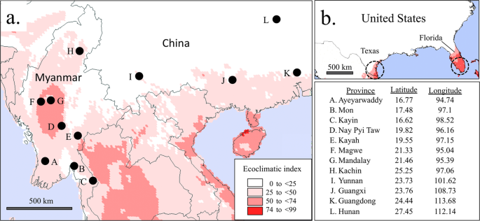
Map and coordinates of collection sites in Myanmar and China combined with CLIMEX modeling of area suitability for fall armyworm. Collection (i) describes pheromone trapping of adult males. All others represent larval collections from corn host plants. (a) locations of sites overlaid on CLIMEX projection of fall armyworm suitability based on calculations of the Ecoclimatic Index (EI), with higher values indicating greater likelihood of persistent fall armyworm populations. (b) CLIMEX projections for the southeastern United States with the same parameters used in Asia. Circles indicate approximate regions where fall armyworm populations are localized during the winter in the United States based on monitoring studies.
Larvae from Myanmar were processed using a 5-ml Dounce homogenizer (Thermo Fisher Scientific, Waltham, MA, USA) in 800 µl Genomic Lysis buffer (Zymo Research, Orange, CA, USA). The homogenate was incubated at 55 °C for 15–30 min, then centrifuged at 10,000 rpm for 5 min. DNA was purified using a Zymo-Spin III column (Zymo Research, Orange, CA, USA) and processed according to manufacturer’s instructions. Genomic DNA preparations were stored at −20 °C. Species identity was initially estimated by larval morphology and confirmed by COI sequence analysis.
Larvae from China were ground with liquid nitrogen and genomic DNAs extracted with Axyprep Multisource Genomic DNA Miniprep Kit (Corning, Corning, NY) according to manufacturer’s instructions. Genomic DNA were stored at −20 °C before analysis. Species were identified according to morphological characteristics.
PCR amplification and DNA sequencing
Polymerase chain reaction (PCR) amplification occurred in a 30 µl reaction mix with a final concentration of 1X ThermoPol reaction buffer and 0.75 units Taq DNA polymerase (both from New England Biolabs, Beverly, MA), 0.17 mM dNTP, and 0.3 µM of each primer. The PCR protocol was 94 °C (1 min), followed by 30 cycles of 92 °C (30 s), 58 °C (30 s), 72 °C (45 s), and a final segment of 72 °C for 3 min. Primers were synthesized by Integrated DNA Technologies (Coralville, IA). Amplification of the COIB segment was done with primers c924F (5′-TTATTGCTGTACCAACAGGT-3′) and c1303R (5′- CAGGATAGTCAGAATATCGACG-3′). Samples that gave poor amplification were reanalyzed using nested PCR in which the first amplification was performed using primers c891F (5′-TACACGAGCATATTTTACATC-3′) and c1472R (5′-GCTGGTGGTAAATTTTGATATC-3′) followed by a second PCR using the internal primers c924F and c1303R. Amplification of the Tpi segment was done with primers t412F (5′- CCGGACTGAAGGTTATCGCTTG -3′) and t1140R (5′- GCGGAAGCATTCGCTGACAACC-3′). Nested PCR was also used, with the first PCR done with primers t634F (5′-TTGCCCATGCTCTTGAGTCC-3′) and t1166R (5′-TGGATACGGACAGCGTTAGC-3′) and the second PCR using the internal primers t412F and t1140R.
For gel electrophoresis, 6 µl of 6X gel loading buffer was added to each amplification reaction and the entire sample run on a 1.8% agarose horizontal gel containing GelGreen (Biotium, Hayward, CA) in 0.5X Tris-borate buffer (TBE, 45 mM Tris base, 45 mM boric acid, 1 mM EDTA pH 8.0). Fragments were visualized on a blue light box and excised from the gel. DNA purification was performed using Zymo-Spin I columns (Zymo Research, Orange, CA) according to manufacturer’s instructions. Genewiz (South Plainfield, NJ) performed the DNA sequencing.
DNA alignments and consensus building were performed using MUSCLE (multiple sequence comparison by log-expectation), a public domain multiple alignment software. Phylogenetic trees were constructed using the Tamura-Nei genetic distance model and the UPGMA tree building network27. These programs are incorporated into the Geneious Pro 10.1.2 program (Biomatters, New Zealand, http://www.geneious.com)28.
Characterization of the COI and Tpi gene segments
The COI and Tpi strain diagnostic markers are single nucleotide substitutions. Site designations begin with an “m” (mitochondria) or “g” (genomic). This is then followed in order by the gene name, number of base pairs from the predicted translational start site (for COI) or the 5′ start of the exon (Tpi), and finally the observed polymorphism using IUPAC convention (R = A or G; Y = C or T; W = A or T; K = G or T; S = C or G; D = A or G or T).
The COIB segment was amplified by primers c924F and c1303R. Species identity of the Myanmar specimens was confirmed by sequence comparisons of COIB259, a 259-bp segment common to the GenBank sequences for the following Spodoptera species, S. abula (HQ177287), S. cosmiodes (HQ177295), S. descoinsi (HQ177306), S. dolichos (HQ177313), S. eridania (Stoll in Cramer)(HQ177321), S. exempta (Walker)(HQ177334), S. exigua (Hübner)(HQ177339), S. latisfscia (Walker)(HQ177354), S. littoralis (Boisduval)(HQ177364), S. mauritia (Boisduval)(HQ177382), S. ornithogalli (Guenée)(HQ177392), S. praefica (Grote)(HQ177407), S. litura (F.)(HQ177375). Sites mCOI1164D and mCOI1287R are diagnostic for strain identity in Western Hemisphere populations where there is a single rice-strain, T1164A1287, and four corn-strain configurations, A1164A1287 (h1), A1164G1287 (h2), G1164A1287 (h3), and G1164G1287 (h4)29 (Fig. 2a).
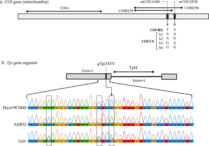
Diagrams of relevant regions in the COI and Tpi genes used for molecular analysis. (a) the COI gene segments with locations of polymorphic sites used for categorizing the COI-CS h1-h4 variants. (b) Map of the Tpi gene segment consisting of the fourth exon of the presumptive open reading frame and adjacent intron. Site gTpi183Y defines the Tpi-based strain identity. Below are chromatographs for the exon segment containing gTpi183Y and two other strain-specific polymorphic sites. Mya1907B40 is a TpiC allele found in Myanmar while AfrRS1 is the TpiR allele identified in Africa. Combining the two produces the overlapping chromatograph pattern found with TpiH.
The Tpi Exon-4 segment consists of multiple strain specific polymorphisms with the gTpi183Y site considered diagnostic of strain identity (Fig. 2b). A C183 identifies the C-strain allele, TpiC, while T183 defines the R-strain, TpiR21. The Tpi gene is located on the Z sex chromosome that is present in one copy in females and two copies in males, with the latter providing opportunities for heterozygosity. Because the genomic DNA was directly sequenced, males heterozygous for Tpi alleles will simultaneously display both alternatives at polymorphic sites, which if different can be identified by overlapping sequencing chromatographs. Heterozygosity at site gTpi183Y gave rise to an overlapping C and T signal at gTpi183Y. This was designated TpiH and defined as representing a TpiC/TpiR heterozygote.
A portion of the adjacent Tpi intron was previously used in phylogenetic comparisons30,31. An approximately 172-bp segment of the intron (TpI4) beginning 10-bp from the 5′ splice site was used in the analysis, with the length variable because of indels. This segment was chosen because it displayed the most consistent sequence quality with the given primers. Many samples examined were heterozygous for frameshift mutations within the intron that produced overlapping chromatographs beginning at the polymorphism. These were not further analyzed. Sequences deposited in GenBank include Mya1907c28 (MN551267), Mya1910a85 (MN551268), Mya1907d14 (MN551269), Mya1910B28 (MN551270), AfrCa1a (MN551271), AfrCa2a (MN551272), AfrCa2b (MN551273), AfrCa1b (MN551274), AfrCa2c (MN551275), and AfrRa1a (MN551276).
Calculation of haplotype numbers
Specimens have a single mitochondrial COI haplotype and so frequency was calculated as the number of specimens with a given COI haplotype divided by the total number of specimens. The Tpi marker is more complicated because of the potential for heterozygosity. Specimens can be characterized by three Tpi strain categories, TpiC (C-strain), TpiR (R-strain), and TpiH (TpiC/TpiR heterozygote). Frequencies at the specimen level were calculated by the number of each category divided by the total number of specimens. We also calculated the frequency of Tpi chromosomes, which allows inclusion of the TpiH specimens when estimating the number of Tpi alleles. Larvae were not sexed so those identified as TpiC or TpiR could have one (females) or two (males) copies of the Tpi gene. We accounted for this uncertainty by assuming a 1:1 sex ratio and using 1.5 as the mean number of Tpi genes per TpiC or TpiR specimen based on the formula of [2 (Tpi genes in males) + 1 (Tpi gene in females)]/2. The TpiH specimens were presumed to carry one copy each of TpiC and TpiR. From these considerations we derived the following formulae, TpiC (chromosomes) = 1.5 X TpiC (specimens) + TpiH and TpiR (chromosomes) = 1.5 X TpiR (specimens) + TpiH. Chromosome frequency was calculated by dividing the number of TpiC or TpiR chromosomes by the total number of chromosomes, as determined by the equation Total chromosomes = 1.5(TpiC + TpiR specimens) + 2(TpiH specimens).
CLIMEX climate suitability analysis
CLIMEX estimates the potential geographical distribution and relative abundance of a species based on biological parameters and regional climate conditions32. The biological parameter values for fall armyworm were previously published (Table 1)33. Climate information was imported from Climond (www.climond.org)32,34 for selected regions using historical data from 1961–1990 at a resolution of 10 feet.
The Ecoclimatic Index (EI) integrates projected growth potential counterbalanced by estimates of stress, the latter of which is based primarily on unfavorable temperature and moisture conditions. EI is presented on a 0–100 scale, where 100 represent continuous 100% suitability (as in an incubator). For this study, the Compare Locations (1 species) function in the CLIMEX program was used with the Grid Data simulation file. No climate change scenario or irrigation components were set. An EI map was created from the simulation.
Source: Ecology - nature.com

